Training Petal Beam

Trains a diffractive optical system to convert a Gaussian beam into an eight-petal beam using a superposition of Laguerre-Gaussian modes.

The three trainable phase modulation layers are optimized jointly with a mode-overlap fidelity loss, which encourages the output field to match the target up to a global phase.

\[\mathcal{L} = 1 - |\langle \psi_{\text{out}} | \psi_{\text{target}} \rangle|^2\]

This inverse-design setup lets the optimizer redistribute both amplitude and phase across the propagation planes.

import matplotlib.animation as animation
import matplotlib.pyplot as plt
import torch
from torch.nn import Parameter

import torchoptics
from torchoptics import Field, System, visualize_tensor
from torchoptics.elements import PhaseModulator
from torchoptics.profiles import gaussian, laguerre_gaussian

Simulation Parameters

Define the grid size and beam properties.

shape = 250  # Grid size (number of points per dimension)
waist_radius = 300e-6  # Waist radius of the Gaussian beam (m)

# Select computation device
device = "cuda" if torch.cuda.is_available() else "cpu"

# Configure torchoptics defaults
torchoptics.set_default_spacing(10e-6)
torchoptics.set_default_wavelength(700e-9)

Target Field: Eight-Petal Beam

The target is an interference pattern formed by the superposition of two Laguerre-Gaussian modes \(\mathrm{LG}_{0}^{+4}\) and \(\mathrm{LG}_{0}^{-4}\), producing an eight-petal intensity distribution.

petal_profile = laguerre_gaussian(shape, p=0, l=4, waist_radius=waist_radius)
petal_profile += laguerre_gaussian(shape, p=0, l=-4, waist_radius=waist_radius)

target_field = Field(petal_profile, z=0.8).normalize().to(device)
visualize_tensor(target_field.intensity(), title="Target Field")

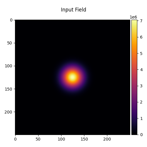
Input Field: Single Gaussian Beam

The input field is a single Gaussian beam at \(z = 0\) m.

input_field = Field(gaussian(shape, waist_radius), z=0).to(device)
visualize_tensor(input_field.intensity(), title="Input Field")

Diffractive Optical System

The system consists of three trainable phase modulation layers.

system = System(
    PhaseModulator(Parameter(torch.zeros(shape, shape)), z=0.2),
    PhaseModulator(Parameter(torch.zeros(shape, shape)), z=0.4),
    PhaseModulator(Parameter(torch.zeros(shape, shape)), z=0.6),
).to(device)

Training Objective

We minimize the mode-overlap fidelity, which reaches zero when the output field matches the target up to a global phase.

Training the System

We optimize the three phase modulators jointly with Adam.

optimizer = torch.optim.Adam(system.parameters(), lr=0.05)
losses = []
frames = []  # Snapshots for animation
num_iterations = 100

for iteration in range(num_iterations):
    optimizer.zero_grad()
    output_field = system.measure_at_z(input_field, 0.8)
    loss = 1 - output_field.inner(target_field).abs().square()
    loss.backward()
    optimizer.step()

    losses.append(loss.item())
    frames.append(
        {
            "iteration": iteration,
            "phases": [elem.phase.detach().cpu().clone() for elem in system.sorted_elements()],  # type: ignore[union-attr]
            "output": output_field.intensity().detach().cpu(),
        }
    )
    if iteration % 20 == 0:
        print(f"Iteration {iteration}, Loss: {losses[-1]:.4f}")

Iteration 0, Loss: 1.0000
Iteration 20, Loss: 0.6290
Iteration 40, Loss: 0.1496
Iteration 60, Loss: 0.0517
Iteration 80, Loss: 0.0313

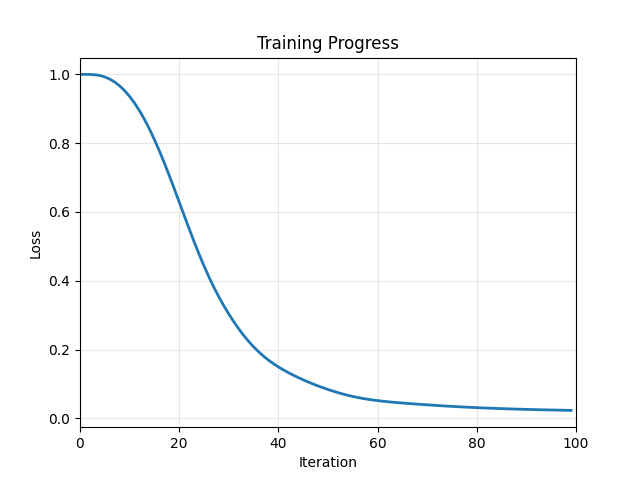
Loss Curve

We plot the fidelity loss to monitor training progress.

plt.plot(losses, linewidth=2)
plt.xlabel("Iteration")
plt.ylabel("Loss")
plt.title("Training Progress")
plt.xlim(0, len(losses))
plt.grid(True, alpha=0.3)
plt.show()

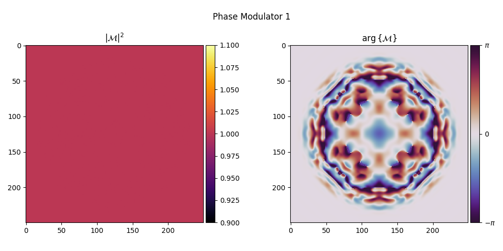
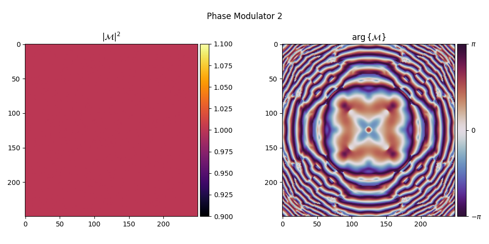
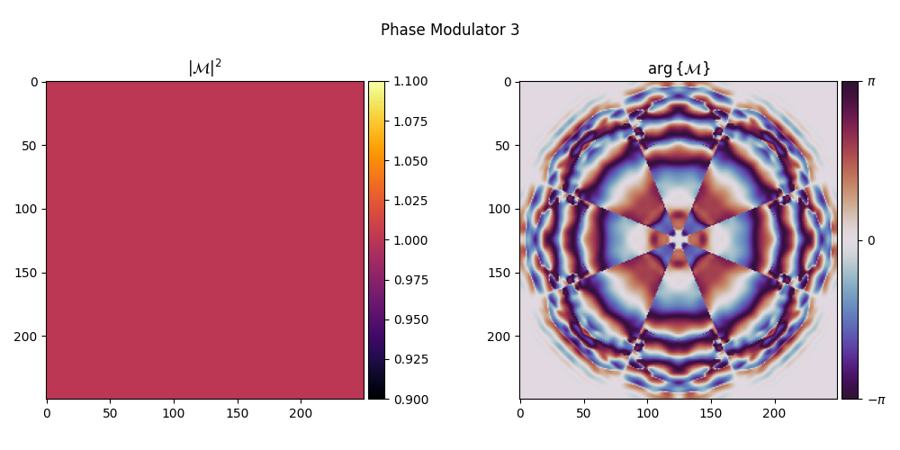
Visualizing the Trained Phase Modulators

We inspect the learned phase modulation layers.

for i, element in enumerate(system):
    element.visualize(title=f"Phase Modulator {i + 1}")

• 
• 
• 

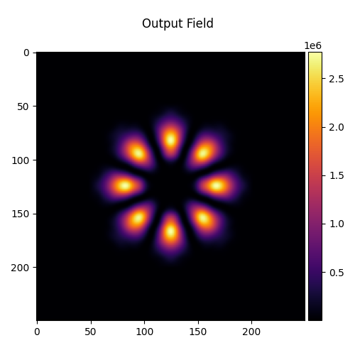
Output Field After Training

Finally, we visualize the trained output alongside the target at \(z = 0.8\) m.

output_field = system.measure_at_z(input_field, 0.8)
visualize_tensor(output_field.intensity(), title="Output Field")

Training Evolution Animation

We animate how the three phase layers, output intensity, and loss evolve over training, with a marker on the loss curve showing progress at each frame.

bounds = input_field.bounds().tolist()
extent = [b * 1e3 for b in bounds]
output_max = max(frame["output"].max().item() for frame in frames)

fig, axes = plt.subplots(
    1, 5, figsize=(18, 3.6), dpi=80, gridspec_kw={"width_ratios": [1, 1, 1, 1, 1.15], "wspace": 0.04}
)
titles = ["Phase Layer 1", "Phase Layer 2", "Phase Layer 3", "Output", "Loss"]

# Phase and intensity panels
ims = []
for i in range(3):
    phase = frames[0]["phases"][i] % (2 * torch.pi)
    im = axes[i].imshow(phase, cmap="twilight", vmin=0, vmax=2 * torch.pi, extent=extent, origin="lower")
    axes[i].set_title(titles[i], fontsize=10)
    axes[i].axis("off")
    ims.append(im)

im_out = axes[3].imshow(
    frames[0]["output"], cmap="inferno", vmin=0, vmax=output_max, extent=extent, origin="lower"
)
axes[3].set_title("Output", fontsize=10)
axes[3].axis("off")

# Loss curve panel
ax_loss = axes[4]
ax_loss.plot(losses, linewidth=1.5)
ax_loss.set_xlim(0, num_iterations)
ax_loss.set_ylim(0, max(losses) * 1.05)
ax_loss.set_xlabel("Iteration", fontsize=9)
ax_loss.set_ylabel("Loss", fontsize=9)
ax_loss.set_title("Loss", fontsize=10)
ax_loss.grid(True, alpha=0.3)
(loss_marker,) = ax_loss.plot([], [], "o", color="#e74c3c", markersize=7, zorder=5)

epoch_text = fig.suptitle("Iteration 0", fontsize=13, fontweight="bold")
fig.subplots_adjust(left=0.02, right=0.98, top=0.86, bottom=0.10, wspace=0.05)


def update(frame_idx):
    frame = frames[frame_idx]
    for i in range(3):
        ims[i].set_data(frame["phases"][i] % (2 * torch.pi))
    im_out.set_data(frame["output"])
    it = frame["iteration"]
    loss_marker.set_data([it], [losses[frame_idx]])
    return ims + [im_out, epoch_text, loss_marker]


anim = animation.FuncAnimation(fig, update, frames=len(frames), interval=100, blit=True)
plt.show()

Once Loop Reflect