Fresnel Zone Plate

Constructs a Fresnel zone plate, a diffractive optical element that focuses light using alternating transparent and opaque concentric rings. The zone boundaries are placed at radii where the optical path difference equals half-wavelength increments:

\[r_n = \sqrt{n \lambda f}\]

where \(n\) is the zone index, \(\lambda\) is the wavelength, and \(f\) is the focal length.

import matplotlib.pyplot as plt
import torch

import torchoptics
from torchoptics import Field, PlanarGrid, System, visualize_tensor
from torchoptics.elements import Modulator

Simulation Parameters

shape = 600  # Grid size (number of points per dimension)
spacing = 5e-6  # Grid spacing (m)
wavelength = 500e-9  # Wavelength (m)
focal_length = 0.3  # Desired focal length (m)

# Configure torchoptics defaults
torchoptics.set_default_spacing(spacing)
torchoptics.set_default_wavelength(wavelength)

# Select computation device
device = "cuda" if torch.cuda.is_available() else "cpu"

Constructing the Zone Plate

We compute the zone plate transmittance by determining which zone each point falls in. Even zones are transparent, odd zones are opaque.

# Create coordinate grid (centered at origin)
xx, yy = PlanarGrid(shape=shape, z=0, spacing=spacing).meshgrid()
r_sq = xx**2 + yy**2

# Zone index: n = r² / (λf)
zone_index = torch.floor(r_sq / (wavelength * focal_length))
zone_plate = (zone_index % 2 == 0).float()

# Number of Fresnel zones within the grid (along the x/y axis, not the diagonal)
half_extent = float(xx.abs().max().item())
n_max = int(half_extent**2 / (wavelength * focal_length))
print(f"Number of Fresnel zones: {n_max}")
print(f"Outermost zone radius: {(n_max * wavelength * focal_length) ** 0.5 * 1e3:.2f} mm")

visualize_tensor(zone_plate, title="Fresnel Zone Plate")

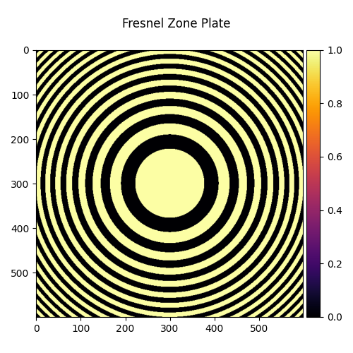
Number of Fresnel zones: 14
Outermost zone radius: 1.45 mm

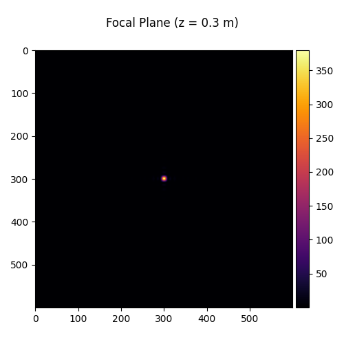
Focusing by the Zone Plate

We illuminate the zone plate with a uniform plane wave and observe the focused intensity at the focal plane.

zone_plate_element = Modulator(zone_plate, z=0).to(device)
system = System(zone_plate_element)

input_field = Field(torch.ones(shape, shape)).to(device)

# Measure at the focal plane
focal_field = system.measure_at_z(input_field, z=focal_length)
visualize_tensor(focal_field.intensity(), title=f"Focal Plane (z = {focal_length} m)")

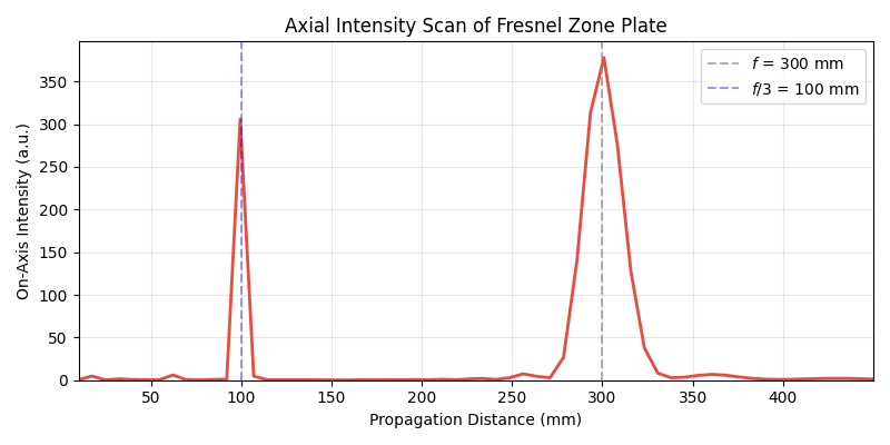
Intensity Along the Optical Axis

We scan the on-axis intensity to verify that the zone plate focuses at the designed focal length \(f\), and also at higher-order foci at \(f/3, f/5, \ldots\) (odd harmonics).

z_scan = torch.linspace(0.01, focal_length * 1.5, 60)
on_axis_intensity = []

for z in z_scan:
    output = system.measure_at_z(input_field, z.item())
    intensity = output.intensity().cpu()
    # On-axis intensity (center pixel)
    on_axis_intensity.append(intensity[shape // 2, shape // 2].item())

fig, ax = plt.subplots(figsize=(8, 4))
ax.plot(z_scan * 1e3, on_axis_intensity, color="#e74c3c", linewidth=2)
ax.axvline(
    focal_length * 1e3, color="gray", linestyle="--", alpha=0.6, label=rf"$f$ = {focal_length * 1e3:.0f} mm"
)
ax.axvline(
    focal_length / 3 * 1e3,
    color="blue",
    linestyle="--",
    alpha=0.4,
    label=rf"$f/3$ = {focal_length / 3 * 1e3:.0f} mm",
)
ax.set_xlabel("Propagation Distance (mm)")
ax.set_ylabel("On-Axis Intensity (a.u.)")
ax.set_title("Axial Intensity Scan of Fresnel Zone Plate")
ax.legend()
ax.set_xlim(z_scan[0].item() * 1e3, z_scan[-1].item() * 1e3)
ax.set_ylim(0)
ax.grid(True, alpha=0.3)
plt.tight_layout()
plt.show()

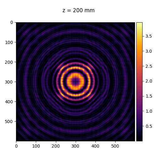
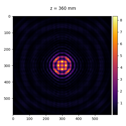
Field at Different Propagation Distances

We visualize the field at several distances to see how the zone plate gradually brings the light to a focus.

distances = [0.1, 0.2, focal_length, focal_length * 1.2]

for z in distances:
    output = system.measure_at_z(input_field, z)
    visualize_tensor(output.intensity(), title=f"z = {z * 1e3:.0f} mm")

• 
• 
• 
•