4f System

Simulates a 4f optical relay, a canonical configuration in Fourier optics that provides access to the spatial frequency spectrum of an input field. Two lenses separated by \(2f\) relay the input to the output while placing the Fourier transform of the field at the midplane. Inserting amplitude masks at this Fourier plane enables spatial filtering: low-pass filters smooth the image, while high-pass filters extract edges and fine detail.

The five key planes have distinct physical meanings:

• \(z = 0\) — Input plane: the object field

• \(z = f\) — Back focal plane of lens 1: spatial frequency spectrum begins forming

• \(z = 2f\) — Fourier plane: exact 2D Fourier transform of the input (spatial filter location)

• \(z = 3f\) — Front focal plane of lens 2

• \(z = 4f\) — Output plane: re-imaged (relay) copy of the input (inverted)

import matplotlib.pyplot as plt
import torch

import torchoptics
from torchoptics import Field, System, visualize_tensor
from torchoptics.elements import Lens, Modulator
from torchoptics.profiles import checkerboard, circle

Simulation Parameters

A checkerboard input field tests both low- and high-frequency response, since a checkerboard contains spatial frequencies near its fundamental tile period.

shape = 500  # Grid size (number of points per dimension)
spacing = 10e-6  # Grid spacing (m)
wavelength = 700e-9  # Wavelength (m)
focal_length = 50e-3  # Lens focal length (m)

tile_length = 200e-6  # Checkerboard tile size (m)
num_tiles = 15  # Number of tiles in each dimension

device = "cuda" if torch.cuda.is_available() else "cpu"

torchoptics.set_default_spacing(spacing)
torchoptics.set_default_wavelength(wavelength)

Input Field: Checkerboard Pattern

The checkerboard provides a rich spatial-frequency test pattern.

field_data = checkerboard(shape, tile_length, num_tiles)
input_field = Field(field_data).to(device)
visualize_tensor(input_field.intensity(), title="Input Field: Checkerboard")

4f Optical System: Key Planes

The unfiltered 4f relay propagates the input to the output without modification (apart from an inversion). We capture the field at the five physically meaningful planes: input (z = 0), back focal plane (z = f), Fourier plane (z = 2f), front focal plane (z = 3f), and output (z = 4f).

fig, axes = plt.subplots(1, 5, figsize=(18, 4.5), constrained_layout=True)
system = System(
    Lens(shape, focal_length, z=1 * focal_length),
    Lens(shape, focal_length, z=3 * focal_length),
).to(device)

for i in range(5):
    plane_z = i * focal_length
    image = system.measure_at_z(input_field, z=plane_z).intensity().cpu()
    axes[i].imshow(image, cmap="inferno", vmin=0, vmax=1)
    axes[i].set_title(f"z = {i}f")
    axes[i].axis("off")
plt.show()

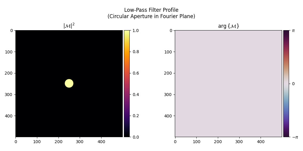
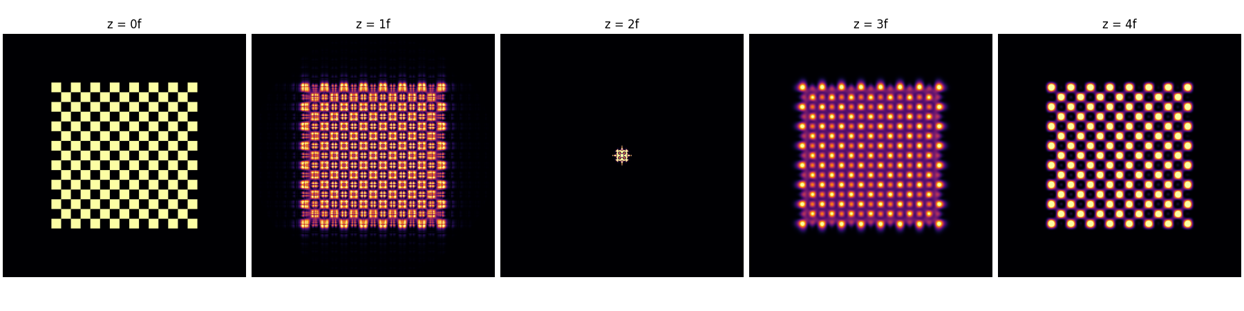
Spatial Filtering: Low-Pass Filter

A circular aperture placed at the Fourier plane (z = 2f) blocks high spatial frequencies, leaving only the low-frequency content. The result is a blurred version of the input; edges are smoothed and fine detail is lost.

radius = 200e-6  # Low-pass filter radius in the Fourier plane (m)
low_pass_profile = circle(shape, radius)

low_pass_4f_system = System(
    Lens(shape, focal_length, z=1 * focal_length),
    Modulator(low_pass_profile, z=2 * focal_length),
    Lens(shape, focal_length, z=3 * focal_length),
).to(device)

low_pass_4f_system[1].visualize(title="Low-Pass Filter Profile\n(Circular Aperture in Fourier Plane)")

fig, axes = plt.subplots(1, 5, figsize=(18, 4.5), constrained_layout=True)
for i in range(5):
    plane_z = i * focal_length
    image = low_pass_4f_system.measure_at_z(input_field, z=plane_z).intensity().cpu()
    axes[i].imshow(image, cmap="inferno", vmin=0, vmax=1)
    axes[i].set_title(f"z = {i}f")
    axes[i].axis("off")
plt.show()

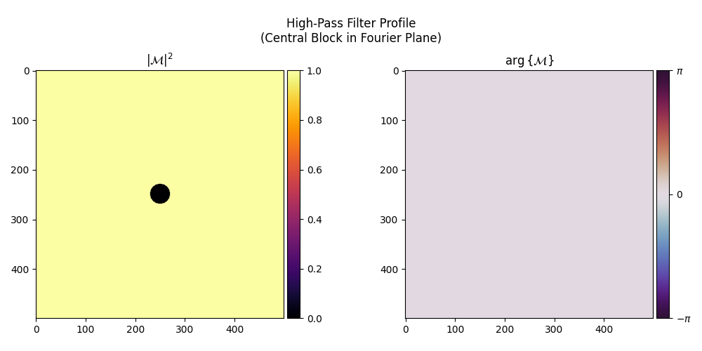
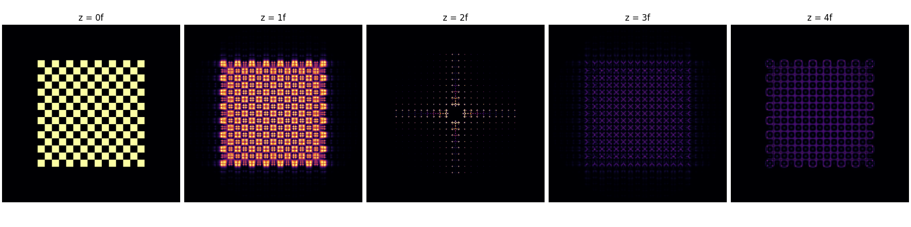
Spatial Filtering: High-Pass Filter

Complementing the low-pass filter, a high-pass filter blocks the central (low-frequency) region of the Fourier plane, retaining only edge and fine-detail information. The result resembles an edge-detected image.

high_pass_profile = 1 - low_pass_profile

high_pass_system = System(
    Lens(shape, focal_length, z=1 * focal_length),
    Modulator(high_pass_profile, z=2 * focal_length),
    Lens(shape, focal_length, z=3 * focal_length),
).to(device)

high_pass_system[1].visualize(title="High-Pass Filter Profile\n(Central Block in Fourier Plane)")

fig, axes = plt.subplots(1, 5, figsize=(18, 4.5), constrained_layout=True)
for i in range(5):
    plane_z = i * focal_length
    image = high_pass_system.measure_at_z(input_field, z=plane_z).intensity().cpu()
    axes[i].imshow(image, cmap="inferno", vmin=0, vmax=1)
    axes[i].set_title(f"z = {i}f")
    axes[i].axis("off")
plt.show()