
Quickstart#
This guide introduces the core workflow of TorchOptics: creating optical fields, propagating them through free space, simulating optical elements, building multi-element systems, and optimizing optical designs using gradient descent.
Before starting, make sure TorchOptics is installed (Installation).
Overview#
TorchOptics simulates optical systems using Fourier optics, where light is modeled as complex-valued wavefronts sampled on 2D grids. Built on PyTorch, every operation is fully differentiable, enabling gradient-based optimization of optical designs.
The library is built around three core abstractions:
Field— A monochromatic optical field: complex-valued data on a 2D planar grid at a position along the optical axis.Element(e.g.,Lens,PhaseModulator) — Optical components that transform fields at specified \(z\) positions.System— An ordered sequence of elements forming a complete optical setup, analogous totorch.nn.Sequential.
Two global defaults set the physical scale of the simulation:
Spacing — Physical distance between adjacent grid points (meters).
Wavelength — Wavelength of the monochromatic light (meters).
Setup#
Import TorchOptics and set the two global defaults (grid spacing and wavelength) that all subsequent fields and elements will inherit:
import torch
import torchoptics
from torchoptics import Field, System
from torchoptics.elements import AmplitudeModulator, Lens
from torchoptics.profiles import checkerboard, circle, gaussian

torchoptics.set_default_spacing(10e-6)       # 10 µm grid spacing
torchoptics.set_default_wavelength(700e-9)   # 700 nm (red light)
Fields and Propagation#
A Field wraps a 2D complex-valued tensor together with its spatial geometry
(grid shape, spacing, offset, and \(z\) position). The torchoptics.profiles module
provides functions for common spatial profiles (Gaussian beams, geometric apertures, gratings, etc.).
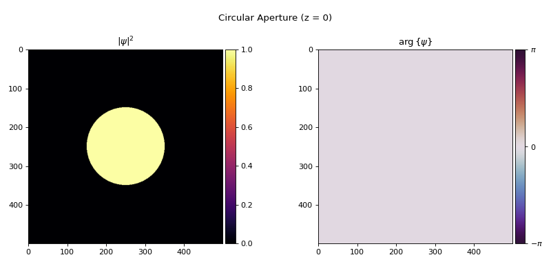
Let’s create a field from a circular aperture:
shape = 500  # 500×500 grid (5 mm × 5 mm physical extent)
field = Field(circle(shape, radius=1e-3))
field.visualize(title="Circular Aperture (z = 0)")
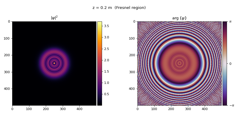
Use propagate_to_z() to propagate a field through free space. As light
travels, it diffracts, producing characteristic patterns at different distances:
# Near-field (Fresnel) diffraction
field.propagate_to_z(0.2).visualize(title="z = 0.2 m  (Fresnel region)")
# Far-field (Fraunhofer) diffraction: the Airy pattern
field.propagate_to_z(2.0).visualize(title="z = 2.0 m  (Fraunhofer region)")
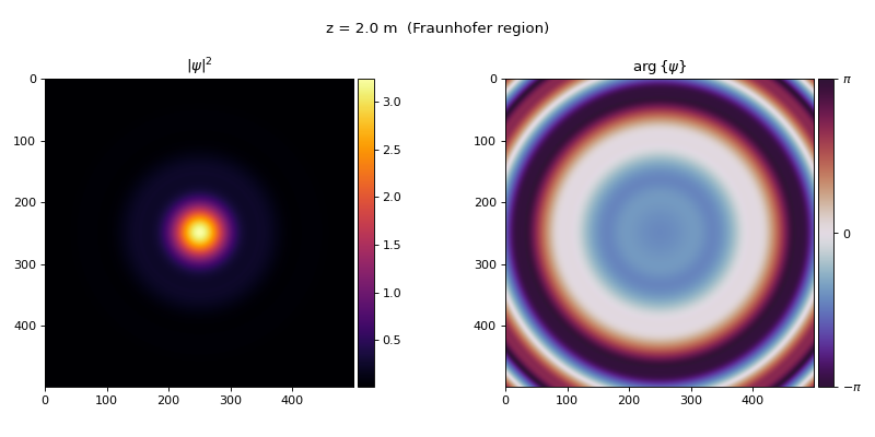
Close to the aperture (the Fresnel region), diffraction produces fringes near the edges. Far away (the Fraunhofer region), the wavefront converges to the Airy pattern, the Fourier transform of the circular aperture.
Note
TorchOptics automatically selects between the angular spectrum method (ASM) and the
direct integration method (DIM) based on the propagation distance and grid geometry.
This can be overridden with the propagation_method parameter.
Focusing with a Lens#
The Lens models a thin lens with focal length \(f\). It applies
a quadratic phase factor with a circular aperture to the incident field:
where \(r = \sqrt{x^2 + y^2}\), \(R\) is the aperture radius (half the lens’s physical extent), \(\lambda\) is the wavelength, and \(f\) is the focal length.
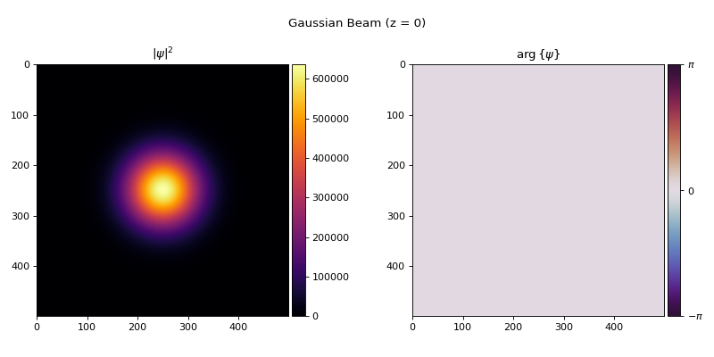
Calling an element on a field (lens(field)) applies this transformation. Let’s focus a Gaussian
beam with a 200 mm lens:
gaussian_beam = Field(gaussian(shape, waist_radius=1e-3))
gaussian_beam.visualize(title="Gaussian Beam (z = 0)")
f = 200e-3  # Focal length: 200 mm
lens = Lens(shape, f, z=0)

focused = lens(gaussian_beam).propagate_to_z(f)
focused.visualize(title=f"Focal Plane (z = {f} m)")
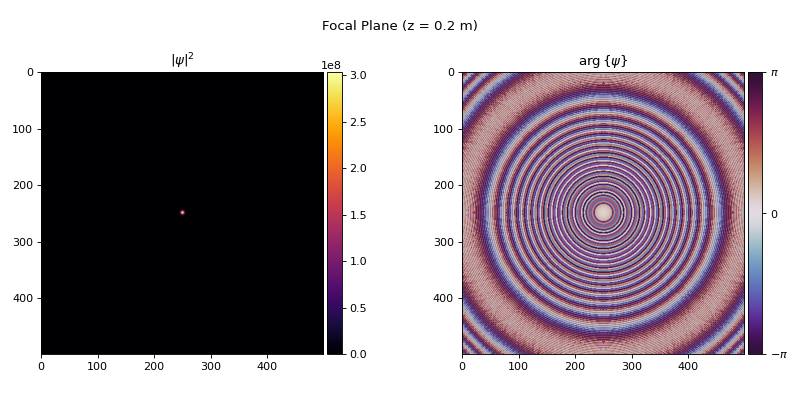
The beam converges to a tight spot at the focal plane.
Optical Systems#
For multi-element setups, the System class handles propagation between
components automatically; you just specify where each element sits along the optical axis.
Use measure_at_z() to compute the field at any \(z\) position.
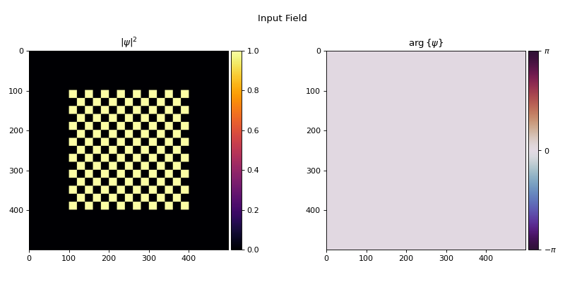
As an example, let’s build a 4f system: two lenses separated by \(2f\) with a spatial filter at the Fourier plane (\(z = 2f\)). The system relays the input image to the output plane (\(z = 4f\)), while the Fourier plane in between gives direct access to the spatial frequency content for filtering. Here we place a high-pass filter that blocks low spatial frequencies, extracting edges from a checkerboard:
input_field = Field(checkerboard(shape, tile_length=200e-6, num_tiles=15))
input_field.visualize(title="Input Field", vmax=1)
# High-pass filter at the Fourier plane (z = 2f)
f = 50e-3  # Focal length: 50 mm
filter_mask = 1 - circle(shape, radius=200e-6)
aperture = AmplitudeModulator(filter_mask, z=2 * f)

aperture.visualize(title="High-Pass Filter at Fourier Plane")
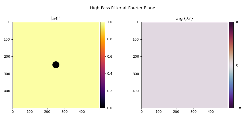
The AmplitudeModulator at the Fourier plane applies a
transmittance mask: 1 - circle(...) blocks the DC and low-frequency components, passing only
the high-frequency content.
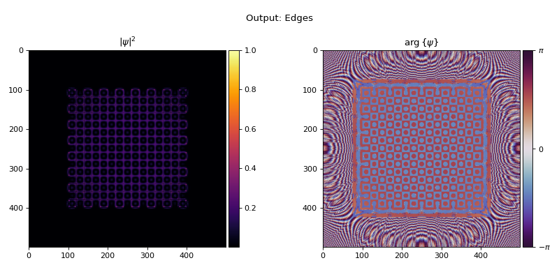
# 4f system with high-pass filter at the Fourier plane
system = System(
    Lens(shape, f, z=1 * f),
    aperture,
    Lens(shape, f, z=3 * f),
)

output = system.measure_at_z(input_field, z=4 * f)
output.visualize(title="Output: Edges", vmax=1)
GPU Acceleration#
All TorchOptics objects are standard PyTorch modules. Move fields and systems to the GPU with
.to() for accelerated computation, especially beneficial for large grids and optimization
loops:
device = "cuda" if torch.cuda.is_available() else "cpu"

field = field.to(device)
system = system.to(device)

output = system.measure_at_z(field, z=4 * f)
Inverse Design#
Every operation in TorchOptics is fully differentiable through torch.autograd. This means
you can optimize optical designs using gradient descent, the same approach used to train neural
networks.
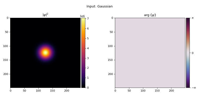
As an example, let’s train a diffractive system to reshape a Gaussian beam into an eight-petal beam. First, we define the input and target fields:
import torch
from torch.nn import Parameter
import torchoptics
from torchoptics import Field, System
from torchoptics.elements import PhaseModulator
from torchoptics.profiles import gaussian, laguerre_gaussian

torchoptics.set_default_spacing(10e-6)
torchoptics.set_default_wavelength(700e-9)

shape = 250
waist_radius = 300e-6

# Input: Gaussian beam
input_field = Field(gaussian(shape, waist_radius=waist_radius), z=0)
input_field.visualize(title="Input: Gaussian")
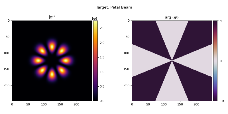
The target is a superposition of two Laguerre-Gaussian modes with opposite orbital angular momentum:
whose interference produces an eight-petal intensity pattern.
# Target: eight-petal beam (LG_0^{+4} + LG_0^{-4} superposition)
target_data = laguerre_gaussian(shape, p=0, l=4, waist_radius=waist_radius) \
            + laguerre_gaussian(shape, p=0, l=-4, waist_radius=waist_radius)
target_field = Field(target_data, z=0.8).normalize()  # normalize to unit power
target_field.visualize(title="Target: Petal Beam")
The loss is \(1 - |\eta|^2\), where \(\eta\) is the inner product (mode overlap) between the output and target fields: equal to 1 when they are identical and 0 when orthogonal.
# Trainable diffractive system: three phase planes initialized to zero
system = System(
    PhaseModulator(Parameter(torch.zeros(shape, shape)), z=0.2),
    PhaseModulator(Parameter(torch.zeros(shape, shape)), z=0.4),
    PhaseModulator(Parameter(torch.zeros(shape, shape)), z=0.6),
)

optimizer = torch.optim.Adam(system.parameters(), lr=0.05)
for iteration in range(200):
    optimizer.zero_grad()
    output = system.measure_at_z(input_field, z=0.8)
    loss = 1 - output.inner(target_field).abs().square()  # 1 - |η|²
    loss.backward()
    optimizer.step()
with torch.no_grad():
    result = system.measure_at_z(input_field, z=0.8)
result.visualize(title="Optimized Output")
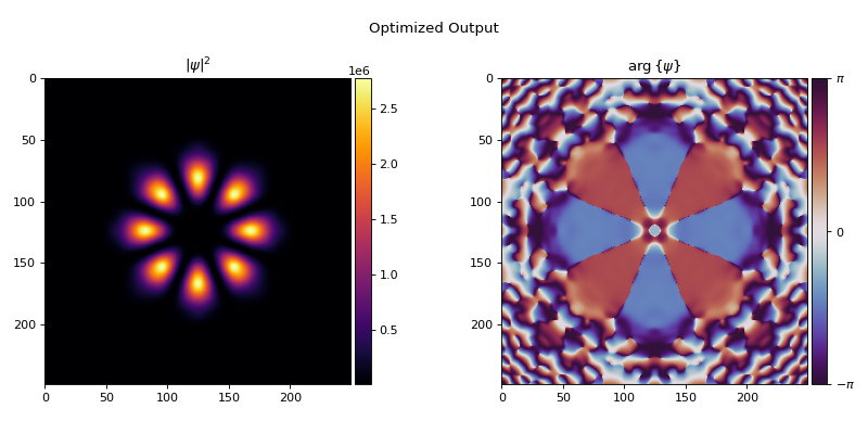
The optimizer discovers the phase patterns that reshape the beam into the target distribution, with no manual optical design required. This approach scales to complex objectives involving multiple elements, custom loss functions, and joint optimization with neural networks.
Tip
See the optimization examples for complete inverse design workflows with loss curves and animations.
Next Steps#
User Guide — In-depth guides on fields, elements, and systems.
Examples — Diffraction, polarization, spatial coherence, and inverse design examples.
API Reference — Complete API documentation.