Gaussian Beam Propagation

Simulates the free-space propagation of a Gaussian beam, the most fundamental solution to the paraxial wave equation. Gaussian beams exhibit a characteristic divergence as they propagate, with the beam waist expanding according to the Rayleigh range.

import matplotlib.pyplot as plt
import torch

import torchoptics
from torchoptics import Field, visualize_tensor
from torchoptics.profiles import gaussian

Simulation Parameters

We define a Gaussian beam with a specified waist radius. The Rayleigh range \(z_R = \pi w_0^2 / \lambda\) is the distance at which the beam radius has grown by a factor of \(\sqrt{2}\).

shape = 256  # Grid size
spacing = 10e-6  # Grid spacing (m)
wavelength = 632.8e-9  # HeNe laser wavelength (m)

waist_radius = 200e-6  # Beam waist radius w_0 (m)
rayleigh_range = torch.pi * waist_radius**2 / wavelength  # z_R (m)

# Configure torchoptics defaults
torchoptics.set_default_spacing(spacing)
torchoptics.set_default_wavelength(wavelength)

device = "cuda" if torch.cuda.is_available() else "cpu"

print(f"Waist radius: {waist_radius * 1e6:.0f} µm")
print(f"Rayleigh range: {rayleigh_range * 1e3:.1f} mm")

Waist radius: 200 µm
Rayleigh range: 198.6 mm

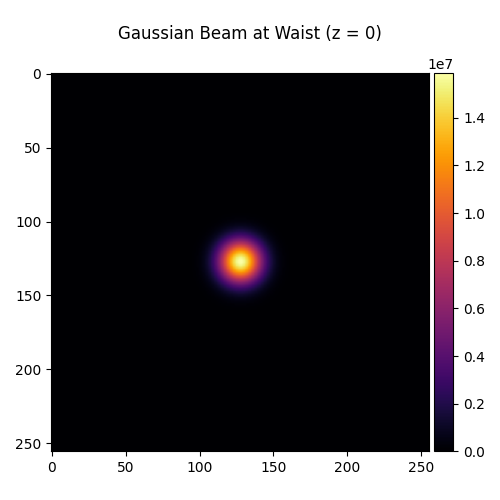
Input Field: Gaussian Beam at Waist

At \(z = 0\) (the beam waist), the Gaussian beam has its minimum radius and a flat phase front.

profile = gaussian(shape, waist_radius=waist_radius)
input_field = Field(profile).to(device)

visualize_tensor(input_field.intensity(), title="Gaussian Beam at Waist (z = 0)")

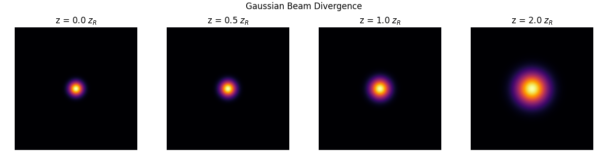
Beam Propagation

As the Gaussian beam propagates, it diverges. The beam radius grows as:

\[w(z) = w_0 \sqrt{1 + (z/z_R)^2}\]

At \(z = z_R\), the beam radius has increased by \(\sqrt{2}\) and the beam area has doubled.

propagation_distances = [0, rayleigh_range / 2, rayleigh_range, 2 * rayleigh_range]

fig, axes = plt.subplots(1, 4, figsize=(12, 3), constrained_layout=True)

for ax, z in zip(axes, propagation_distances):
    output_field = input_field.propagate_to_z(z)
    intensity = output_field.intensity().cpu()
    ax.imshow(intensity, cmap="inferno")
    ax.set_title(f"z = {z / rayleigh_range:.1f} $z_R$")
    ax.axis("off")

plt.suptitle("Gaussian Beam Divergence")
plt.show()

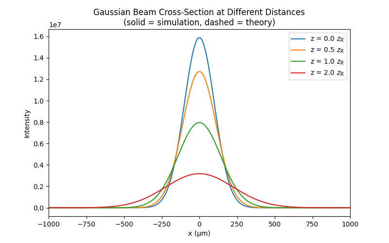
Intensity Cross-Section

We plot the horizontal intensity profile at different propagation distances. The beam maintains its Gaussian shape but broadens as it propagates.

fig, ax = plt.subplots(figsize=(8, 5))
x = torch.linspace(-shape // 2 * spacing, shape // 2 * spacing, shape) * 1e6  # µm
x_fine = torch.linspace(-shape // 2 * spacing, shape // 2 * spacing, 500) * 1e6  # µm

for z in propagation_distances:
    output_field = input_field.propagate_to_z(z)
    intensity = output_field.intensity().cpu()
    cross_section = intensity[shape // 2, :]
    (line,) = ax.plot(x, cross_section, label=f"z = {z / rayleigh_range:.1f} $z_R$")

    # Overlay the theoretical Gaussian profile w(z) = w_0 * sqrt(1 + (z/z_R)^2)
    w_z = waist_radius * (1 + (z / rayleigh_range) ** 2) ** 0.5
    I_peak = cross_section.max().item()
    I_theory = I_peak * torch.exp(-2 * (x_fine * 1e-6) ** 2 / w_z**2)
    ax.plot(x_fine, I_theory, "--", color=line.get_color(), alpha=0.55, linewidth=1.2)

ax.set_xlabel("x (µm)")
ax.set_ylabel("Intensity")
ax.set_title("Gaussian Beam Cross-Section at Different Distances\n(solid = simulation, dashed = theory)")
ax.legend()
ax.set_xlim(-1000, 1000)
plt.show()