Talbot Effect

Demonstrates the Talbot effect, the self-imaging of periodic structures through free-space propagation. When a periodic grating is illuminated by a coherent plane wave, exact replicas of the grating appear at multiples of the Talbot distance:

\[z_T = \frac{2 d^2}{\lambda}\]

where \(d\) is the grating period and \(\lambda\) is the wavelength. At half the Talbot distance, a laterally shifted copy appears.

import matplotlib.pyplot as plt
import torch

import torchoptics
from torchoptics import Field, visualize_tensor
from torchoptics.profiles import binary_grating, gaussian

Simulation Parameters

We define a binary grating and compute the Talbot distance.

shape = 300  # Grid size (number of points per dimension)
spacing = 5e-6  # Grid spacing (m)
wavelength = 500e-9  # Wavelength (m), green light
grating_period = 50e-6  # Grating period (m)
# Talbot distance
z_talbot = 2 * grating_period**2 / wavelength
print(f"Talbot distance: z_T = {z_talbot * 1e3:.1f} mm")

# Configure torchoptics defaults
torchoptics.set_default_spacing(spacing)
torchoptics.set_default_wavelength(wavelength)

# Select computation device
device = "cuda" if torch.cuda.is_available() else "cpu"

Talbot distance: z_T = 10.0 mm

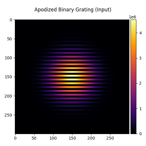
Input Field: Binary Grating

We create a binary amplitude grating as the input field.

grating = binary_grating(shape, grating_period)

# Apply a Gaussian apodization envelope to smoothly suppress hard aperture edges,
# which otherwise cause strong diffraction artefacts that obscure the Talbot pattern.
waist_radius = 0.25 * shape * spacing  # 25% of aperture width
envelope = gaussian(shape, waist_radius).abs()
input_field = Field(grating * envelope).to(device)
visualize_tensor(input_field.intensity(), title="Apodized Binary Grating (Input)")

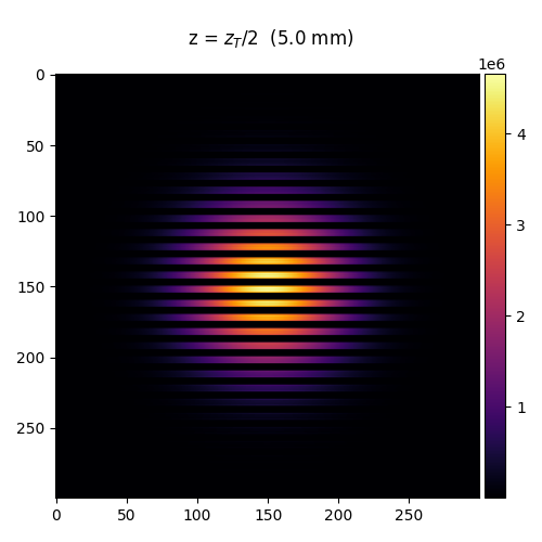
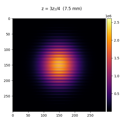
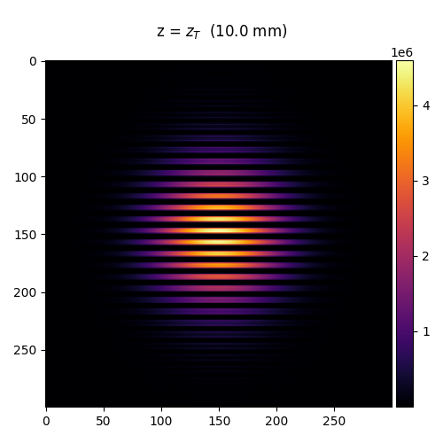
Self-Imaging at Talbot Distances

We propagate the field to key fractional Talbot distances:

• \(z = z_T/4\): fractional Talbot image (doubled frequency)

• \(z = z_T/2\): shifted self-image (half-period lateral shift)

• \(z = 3z_T/4\): complementary fractional image

• \(z = z_T\): exact self-image

fractional_distances = {
    "$z_T/4$": z_talbot / 4,
    "$z_T/2$": z_talbot / 2,
    "$3z_T/4$": 3 * z_talbot / 4,
    "$z_T$": z_talbot,
}

for label, z in fractional_distances.items():
    output_field = input_field.propagate_to_z(z)
    visualize_tensor(output_field.intensity(), title=f"z = {label}  ({z * 1e3:.1f} mm)")

• 
• 
• 
• 

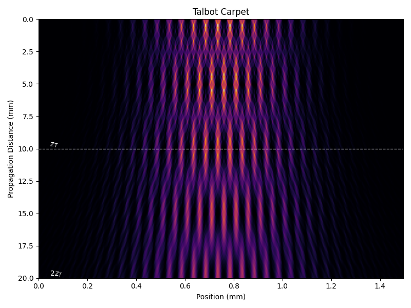
Talbot Carpet

The Talbot carpet is a cross-sectional view of the intensity distribution as a function of propagation distance, revealing the fractal-like self-imaging structure. We propagate the grating through two Talbot distances and collect 1D intensity profiles.

num_z_steps = 200
z_values = torch.linspace(0, 2 * z_talbot, num_z_steps)

# Collect center-column cross-sections
carpet = torch.zeros(num_z_steps, shape)
for i, z in enumerate(z_values):
    output_field = input_field.propagate_to_z(z.item())
    carpet[i] = output_field.intensity().cpu()[:, shape // 2]

Visualize the Talbot carpet

fig, ax = plt.subplots(figsize=(8, 6))
extent = (0, (shape - 1) * spacing * 1e3, 2 * z_talbot * 1e3, 0)
ax.imshow(carpet, cmap="inferno", aspect="auto", extent=extent)
ax.set_xlabel("Position (mm)")
ax.set_ylabel("Propagation Distance (mm)")
ax.set_title("Talbot Carpet")

# Mark Talbot distances
for n, label in [(1, r"$z_T$"), (2, r"$2z_T$")]:
    ax.axhline(y=n * z_talbot * 1e3, color="white", linestyle="--", alpha=0.6, linewidth=1)
    ax.text(
        0.02,
        n * z_talbot * 1e3,
        f"  {label}",
        color="white",
        fontsize=10,
        va="bottom",
        ha="left",
        transform=ax.get_yaxis_transform(),
    )

plt.tight_layout()
plt.show()