Polychromatic Light with Grating

Simulates the propagation of red, green, and blue (RGB) light through a blazed grating, demonstrating wavelength-dependent diffraction, the physical basis of spectroscopy, prism effects, and color separation in optical instruments.

The grating equation governs the diffraction angle \(\theta_m\) of the \(m\)-th diffraction order for a grating with period \(d\):

\[d \sin\theta_m = m \lambda\]

A blazed grating is designed to concentrate light into a particular order by matching the blaze condition. Because longer wavelengths diffract more strongly, a polychromatic beam is spatially dispersed with red farther from the optical axis than blue (for \(m = 1\)).

import matplotlib.pyplot as plt
import torch
from matplotlib.colors import LinearSegmentedColormap

import torchoptics
from torchoptics import Field, System
from torchoptics.elements import PolychromaticPhaseModulator
from torchoptics.profiles import blazed_grating, gaussian

Simulation Parameters

We model three wavelengths corresponding to blue, green, and red light. The blazed grating period sets the scale of angular dispersion.

shape = 500  # Grid size (number of points per dimension)
spacing = 10e-6  # Grid spacing (m)
waist_radius = 300e-6  # Input Gaussian beam waist (m)

wavelengths = [450e-9, 550e-9, 700e-9]  # Blue, green, red (m)
colors = ["blue", "green", "red"]
labels = ["Blue (450 nm)", "Green (550 nm)", "Red (700 nm)"]

grating_period = 100e-6  # Grating period d (m)
blaze_wavelength = wavelengths[0]  # Blaze condition optimized for blue

# Configure torchoptics defaults (spacing only; wavelength set per-field)
torchoptics.set_default_spacing(spacing)

device = "cuda" if torch.cuda.is_available() else "cpu"

# Theoretical first-order deflection angles (radians)
theta_theory = [wl / grating_period for wl in wavelengths]
print("Theoretical first-order diffraction angles:")
for lbl, theta in zip(labels, theta_theory):
    print(f"  {lbl}: {theta * 1e3:.2f} mrad")

Theoretical first-order diffraction angles:
  Blue (450 nm): 4.50 mrad
  Green (550 nm): 5.50 mrad
  Red (700 nm): 7.00 mrad

Input: Polychromatic Gaussian Beam

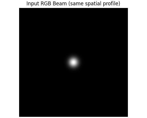
We create a separate Field for each wavelength, all with the same spatial profile.

gaussian_data = gaussian(shape, waist_radius)

fields = [Field(gaussian_data, wavelength=wl).to(device) for wl in wavelengths]


def compose_rgb(channels: list[torch.Tensor]) -> torch.Tensor:
    """Compose a display RGB image from wavelength-ordered channels (blue, green, red)."""
    rgb = torch.stack([channels[2], channels[1], channels[0]], dim=-1)
    return (rgb / rgb.max()).clamp(0, 1)


# Visualize the input (RGB composite)
rgb_norm = compose_rgb([f.intensity().cpu() for f in fields])

fig, ax = plt.subplots(figsize=(5, 4), constrained_layout=True)
ax.imshow(rgb_norm.clamp(0, 1))
ax.set_title("Input RGB Beam (same spatial profile)")
ax.axis("off")
plt.show()

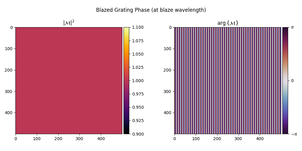
Blazed Grating Phase Modulator

A blazed grating is a surface-relief element whose sawtooth thickness profile imparts a wavelength-dependent phase. The PolychromaticPhaseModulator takes the physical thickness and a refractive index, then evaluates (2π/λ)(n − 1) t(x, y) independently for each field’s wavelength. With n=2 and height = blaze_wavelength, the accumulated phase is exactly 2π at the blaze wavelength, the condition for maximum first-order efficiency.

grating_thickness = blazed_grating(shape, grating_period, height=blaze_wavelength, theta=torch.pi / 2)
system = System(PolychromaticPhaseModulator(grating_thickness, n=2)).to(device)

# Visualize the grating phase at the blaze wavelength
system[0].visualize(wavelength=blaze_wavelength, title="Blazed Grating Phase (at blaze wavelength)")

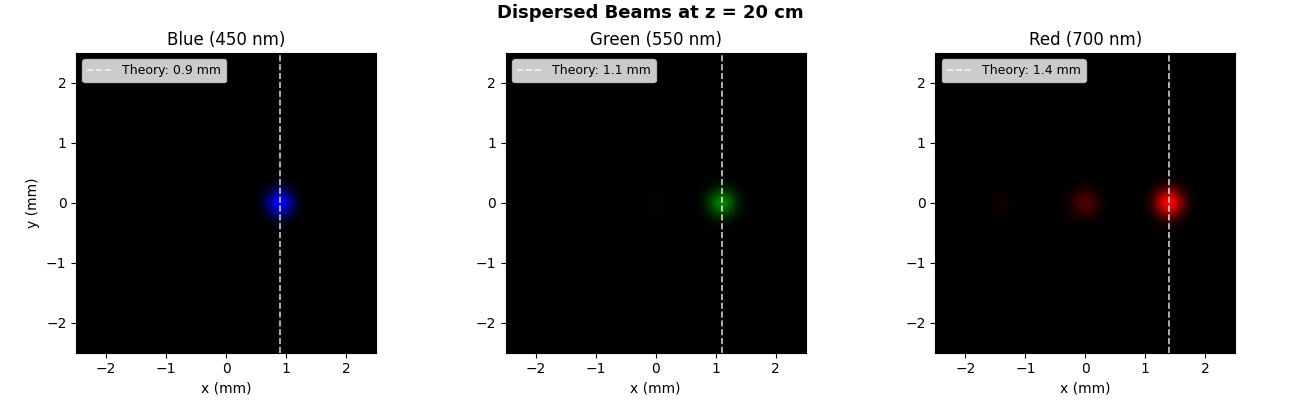
Dispersion at a Fixed Propagation Distance

After propagating a distance z, the first-order spot for each wavelength is laterally displaced by approximately \(\Delta x \approx z \tan\theta_1 \approx z\lambda/d\).

z_observe = 0.2  # Propagation distance (m)

fig, axes = plt.subplots(1, 3, figsize=(13, 4), constrained_layout=True)

x_axis = torch.linspace(-shape * spacing / 2, shape * spacing / 2, shape) * 1e3  # mm

for ax, field, lbl, color, theta in zip(axes, fields, labels, colors, theta_theory):
    output = system.measure_at_z(field, z_observe)
    intensity = output.intensity().cpu()

    cmap = LinearSegmentedColormap.from_list(color, ["black", color])
    ax.imshow(
        intensity,
        cmap=cmap,
        extent=[-shape * spacing / 2 * 1e3, shape * spacing / 2 * 1e3] * 2,
    )
    # Mark expected first-order position
    x_expected = z_observe * theta * 1e3  # mm
    ax.axvline(
        x_expected,
        color="white",
        linestyle="--",
        alpha=0.8,
        linewidth=1.2,
        label=f"Theory: {x_expected:.1f} mm",
    )
    ax.set_title(lbl)
    ax.set_xlabel("x (mm)")
    if ax == axes[0]:
        ax.set_ylabel("y (mm)")
    ax.legend(fontsize=9)

plt.suptitle(f"Dispersed Beams at z = {z_observe * 1e2:.0f} cm", fontsize=13, fontweight="bold")
plt.show()

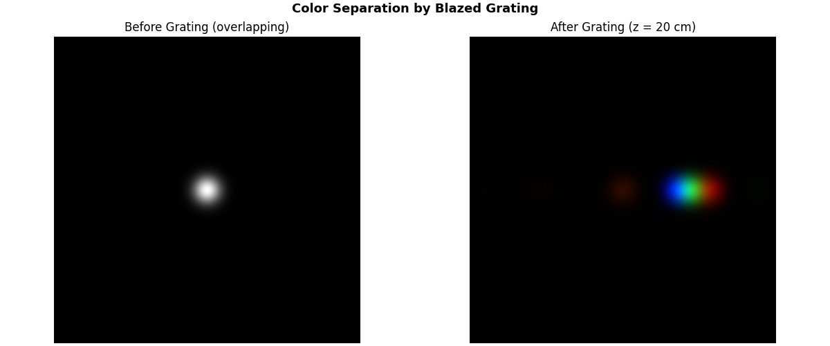
RGB Composite: Color Separation

Overlaying all three channels shows the spatial color separation produced by the grating. Blue is deflected least; red most.

fig, axes = plt.subplots(1, 2, figsize=(12, 5), constrained_layout=True)

# Input composite (before grating)
input_rgb = compose_rgb([f.intensity().cpu() for f in fields])
axes[0].imshow(input_rgb)
axes[0].set_title("Before Grating (overlapping)")
axes[0].axis("off")

# Output composite (after grating + propagation)
out_rgb = compose_rgb([system.measure_at_z(f, z_observe).intensity().cpu() for f in fields])
axes[1].imshow(out_rgb)
axes[1].set_title(f"After Grating (z = {z_observe * 1e2:.0f} cm)")
axes[1].axis("off")

plt.suptitle("Color Separation by Blazed Grating", fontsize=13, fontweight="bold")
plt.show()