
Note
Go to the end to download the full example code.
Young’s Double Slit#
Simulates Young’s double-slit experiment, one of the most iconic demonstrations of wave interference in physics. A coherent beam illuminates two narrow slits, producing an interference pattern on a distant screen that reveals the wave nature of light.
import matplotlib.pyplot as plt
import torch

import torchoptics
from torchoptics import Field, visualize_tensor
from torchoptics.profiles import rectangle
Simulation Parameters#
We define the slit geometry, grid properties, and propagation distances.
shape = 500  # Grid size (number of points per dimension)
spacing = 5e-6  # Grid spacing (m)
wavelength = 500e-9  # Wavelength (m), green light

slit_width = 40e-6  # Width of each slit (m)
slit_height = 1.5e-3  # Height of each slit (m)
slit_separation = 250e-6  # Center-to-center separation (m)

# Configure torchoptics defaults
torchoptics.set_default_spacing(spacing)
torchoptics.set_default_wavelength(wavelength)

# Select computation device
device = "cuda" if torch.cuda.is_available() else "cpu"
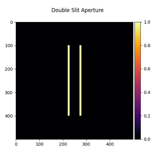
Input Field: Double Slit Aperture#
We create two narrow rectangular slits separated by slit_separation.
The input field is a uniform plane wave transmitted through the two slits.
slit1 = rectangle(shape, side=(slit_height, slit_width), offset=(0, -slit_separation / 2))
slit2 = rectangle(shape, side=(slit_height, slit_width), offset=(0, slit_separation / 2))
aperture = slit1 + slit2

input_field = Field(aperture).to(device)
visualize_tensor(input_field.intensity(), title="Double Slit Aperture")
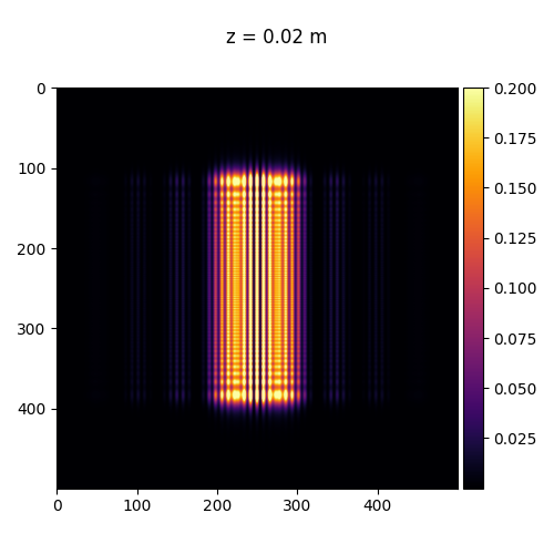
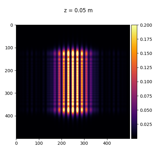
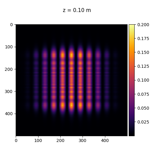
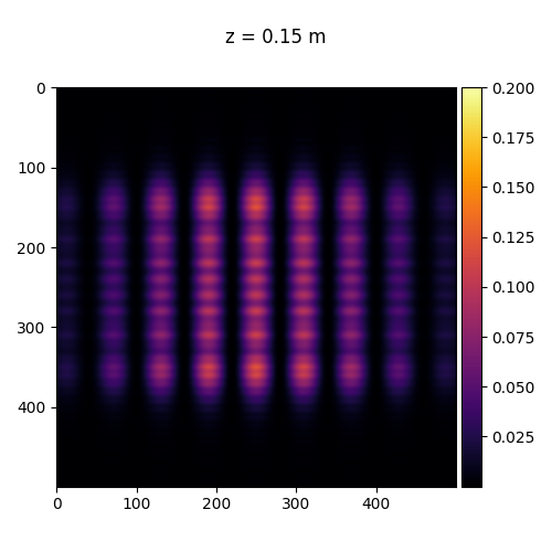
Interference Pattern at Different Distances#
As the field propagates, the waves from the two slits overlap and interfere. The fringe spacing increases with propagation distance according to:
where \(d\) is the slit separation and \(z\) is the propagation distance.
propagation_distances = [0.02, 0.05, 0.1, 0.15]

for z in propagation_distances:
    output_field = input_field.propagate_to_z(z)
    visualize_tensor(output_field.intensity(), title=f"z = {z:.2f} m", vmax=0.2)
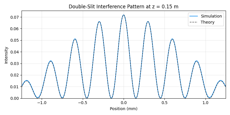
Intensity Cross-Section#
We plot the horizontal intensity profile at the screen, showing the characteristic double-slit interference fringes modulated by the single-slit diffraction envelope.
z_screen = 0.15  # Screen distance (m)
output_field = input_field.propagate_to_z(z_screen)
intensity = output_field.intensity().cpu()

# Take center row cross-section
center_row = intensity[shape // 2, :]
x = torch.linspace(-spacing * (shape - 1) / 2, spacing * (shape - 1) / 2, shape)

# Theoretical pattern: sinc² (single-slit envelope) × cos² (double-slit fringes)
x_theory = torch.linspace(x[0], x[-1], 2000)
u = torch.pi * slit_width * x_theory / (wavelength * z_screen)
v = torch.pi * slit_separation * x_theory / (wavelength * z_screen)
sinc2 = (torch.where(u.abs() < 1e-9, torch.ones_like(u), torch.sin(u) / u)) ** 2
I_theory = sinc2 * torch.cos(v) ** 2
I_theory = I_theory * center_row.max() / I_theory.max()

fig, ax = plt.subplots(figsize=(8, 4))
ax.plot(x * 1e3, center_row, color="#2196F3", linewidth=1.5, label="Simulation")
ax.plot(x_theory * 1e3, I_theory, "k--", linewidth=1.2, alpha=0.7, label="Theory")
ax.set_xlabel("Position (mm)")
ax.set_ylabel("Intensity")
ax.set_title(f"Double-Slit Interference Pattern at z = {z_screen} m")
ax.set_xlim(float(x[0]) * 1e3, float(x[-1]) * 1e3)
ax.set_ylim(0)
ax.legend()
ax.grid(True, alpha=0.3)
plt.tight_layout()
plt.show()
Total running time of the script: (0 minutes 1.577 seconds)