Mach-Zehnder Interferometer

Simulates a Mach-Zehnder interferometer using beam splitter elements. The interferometer splits a beam into two arms, introduces a phase difference in one arm, and recombines them to produce interference. This classic configuration is fundamental to precision measurement, optical sensing, and quantum optics.

import matplotlib.pyplot as plt
import torch

import torchoptics
from torchoptics import Field, visualize_tensor
from torchoptics.elements import BeamSplitter
from torchoptics.profiles import gaussian

Simulation Parameters

shape = 400  # Grid size (number of points per dimension)
spacing = 10e-6  # Grid spacing (m)
wavelength = 700e-9  # Wavelength (m)
waist_radius = 800e-6  # Gaussian beam waist (m)

# Configure torchoptics defaults
torchoptics.set_default_spacing(spacing)
torchoptics.set_default_wavelength(wavelength)

Interferometer Components

A Mach-Zehnder interferometer consists of two 50:50 beam splitters. The dielectric beam splitter has \(\theta = \pi/4\) and zero phase shifts.

bs1 = BeamSplitter(shape, theta=torch.pi / 4, phi_0=0, phi_r=0, phi_t=0)
bs2 = BeamSplitter(shape, theta=torch.pi / 4, phi_0=0, phi_r=0, phi_t=0)

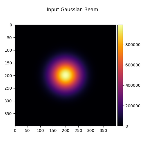
# Input: Gaussian beam
input_field = Field(gaussian(shape, waist_radius))
visualize_tensor(input_field.intensity(), title="Input Gaussian Beam")

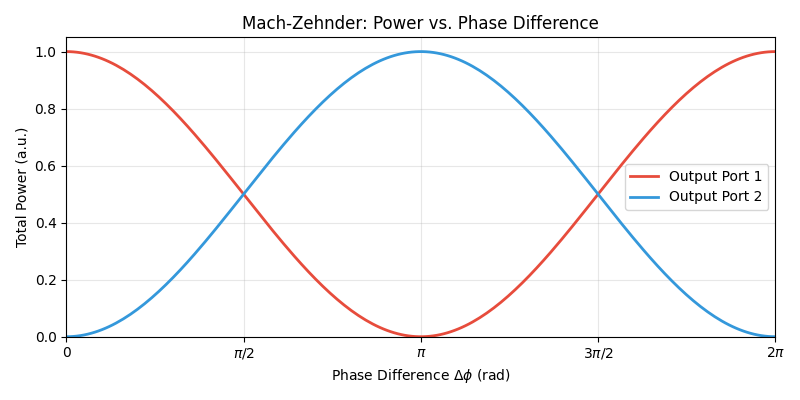
Uniform Phase Sweep

We sweep a uniform phase difference \(\Delta\phi\) in one arm from 0 to \(2\pi\) and observe how the output power oscillates sinusoidally, demonstrating constructive and destructive interference.

The output intensity follows:

\[I_{\text{out}} = \frac{I_0}{2}\left(1 + \cos(\Delta\phi)\right)\]

num_phases = 200
phase_values = torch.linspace(0, 2 * torch.pi, num_phases)
port1_power = []
port2_power = []

for phi in phase_values:
    # Split
    arm1, arm2 = bs1(input_field)

    # Phase shift in arm 2
    arm2 = arm2.modulate(torch.exp(1j * phi) * torch.ones(shape, shape))

    # Recombine
    out1, out2 = bs2(arm1, arm2)

    port1_power.append(out1.power().sum().item())
    port2_power.append(out2.power().sum().item())

fig, ax = plt.subplots(figsize=(8, 4))
ax.plot(phase_values, port1_power, label="Output Port 1", color="#e74c3c", linewidth=2)
ax.plot(phase_values, port2_power, label="Output Port 2", color="#3498db", linewidth=2)
ax.set_xlabel(r"Phase Difference $\Delta\phi$ (rad)")
ax.set_ylabel("Total Power (a.u.)")
ax.set_title("Mach-Zehnder: Power vs. Phase Difference")
ax.set_xticks([0, torch.pi / 2, torch.pi, 3 * torch.pi / 2, 2 * torch.pi])
ax.set_xticklabels(["0", r"$\pi/2$", r"$\pi$", r"$3\pi/2$", r"$2\pi$"])
ax.legend()
ax.set_xlim(0, 2 * torch.pi)
ax.set_ylim(0)
ax.grid(True, alpha=0.3)
plt.tight_layout()
plt.show()

Power Conservation

In an ideal interferometer, total output power equals input power regardless of the phase setting — interference redistributes power between ports, not creates or destroys it. We verify this numerically.

input_power = input_field.power().item()
total_power = [p1 + p2 for p1, p2 in zip(port1_power, port2_power)]
print(f"Input power:                  {input_power:.6f}")
print(f"Total output power (min/max): {min(total_power):.6f} / {max(total_power):.6f}")

Input power:                  0.999999
Total output power (min/max): 0.999999 / 0.999999