Quantum State Discrimination

Demonstrates minimum-error discrimination between two non-orthogonal quantum states encoded in Hermite-Gaussian spatial modes. Because the states are non-orthogonal, perfect discrimination is impossible. We compute the Helstrom bound (the minimum error probability achievable by any measurement) and compare it to the error from direct intensity detection.

import math

import matplotlib.pyplot as plt
import torch

import torchoptics
from torchoptics import Field
from torchoptics.profiles import hermite_gaussian

Simulation Parameters

shape = 300  # Grid size (number of points per dimension)
waist_radius = 300e-6  # Beam waist radius (m)
spacing = 10e-6  # Grid spacing (m)
wavelength = 700e-9  # Wavelength (m)

torchoptics.set_default_spacing(spacing)
torchoptics.set_default_wavelength(wavelength)

Build the Two Quantum States

We define two states as superpositions of Hermite-Gaussian modes:

\[|\psi_1\rangle = |\mathrm{HG}_{00}\rangle, \qquad |\psi_2\rangle = \cos\frac{\pi}{3}\,|\mathrm{HG}_{00}\rangle + \sin\frac{\pi}{3}\,|\mathrm{HG}_{01}\rangle\]

Their overlap is \(|\langle\psi_1|\psi_2\rangle| = \tfrac{1}{2}\), so perfect discrimination is impossible.

hg00 = hermite_gaussian(shape, m=0, n=0, waist_radius=waist_radius)
hg01 = hermite_gaussian(shape, m=0, n=1, waist_radius=waist_radius)

psi1 = Field(hg00, wavelength=wavelength, spacing=spacing)
psi2 = Field(
    math.cos(math.pi / 3) * hg00 + math.sin(math.pi / 3) * hg01,
    wavelength=wavelength,
    spacing=spacing,
)

Inner Product and Helstrom Bound

The Helstrom bound gives the lowest error probability achievable by any measurement (for equal priors \(p_1 = p_2 = \tfrac{1}{2}\)):

\[P_{\mathrm{err}}^{\min} = \frac{1}{2}\Bigl(1 - \sqrt{1 - |\langle\psi_1|\psi_2\rangle|^{2}}\Bigr)\]

overlap = psi1.inner(psi2).abs().item()
helstrom = 0.5 * (1 - (1 - overlap**2) ** 0.5)

print(f"|⟨ψ₁|ψ₂⟩|  = {overlap:.4f}")
print(f"Helstrom bound  P_err^min = {helstrom:.4f}")

|⟨ψ₁|ψ₂⟩|  = 0.5000
Helstrom bound  P_err^min = 0.0670

Direct Detection Error

Direct (intensity) detection assigns each point to the state with higher local intensity. The error probability (equal priors) is:

\[P_{\mathrm{err}}^{x} = \frac{1}{2} \int \min\bigl(|\psi_1(\mathbf{r})|^{2},\; |\psi_2(\mathbf{r})|^{2}\bigr)\,d\mathbf{r}\]

I1 = psi1.intensity()
I2 = psi2.intensity()
cell_area = spacing**2
direct_err = 0.5 * (torch.min(I1, I2).sum() * cell_area).item()
gap = direct_err / helstrom

print(f"Direct detection P_err^x  = {direct_err:.4f}")
print(f"Gap (direct / Helstrom)   = {gap:.1f}×")

Direct detection P_err^x  = 0.2614
Gap (direct / Helstrom)   = 3.9×

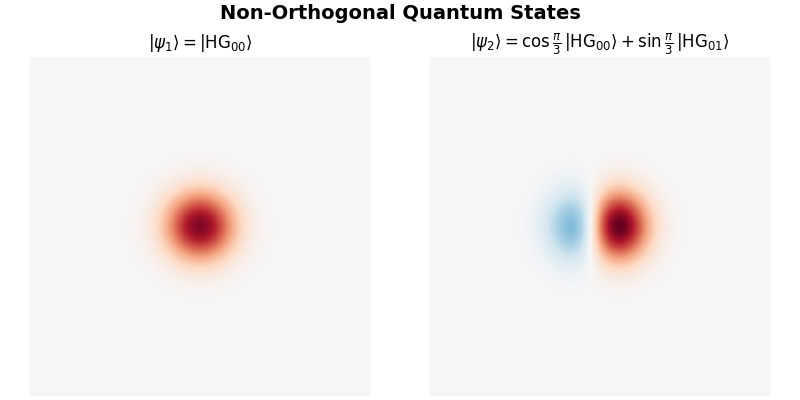
Visualize the States

The real part of each field shows the spatial mode structure. \(|\psi_1\rangle\) is a pure Gaussian, while \(|\psi_2\rangle\) has a two-lobed structure from the \(\mathrm{HG}_{01}\) component.

fig, axes = plt.subplots(1, 2, figsize=(8, 4), constrained_layout=True)
fig.suptitle("Non-Orthogonal Quantum States", fontsize=14, fontweight="bold")

labels = [
    r"$|\psi_1\rangle = |\mathrm{HG}_{00}\rangle$",
    r"$|\psi_2\rangle = \cos\frac{\pi}{3}\,|\mathrm{HG}_{00}\rangle"
    r" + \sin\frac{\pi}{3}\,|\mathrm{HG}_{01}\rangle$",
]
vmax = max(f.data.real.abs().max().item() for f in [psi1, psi2])
for ax, field, label in zip(axes, [psi1, psi2], labels):
    ax.imshow(field.data.real, cmap="RdBu_r", vmin=-vmax, vmax=vmax)
    ax.set_title(label, fontsize=12)
    ax.axis("off")

plt.show()

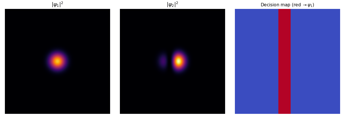
Intensities and Decision Regions

The decision map shows which state is assigned at each spatial point under direct detection. The large overlap between the two intensity profiles explains why direct detection performs poorly.

fig, axes = plt.subplots(1, 3, figsize=(12, 4), constrained_layout=True)

Imax = max(I1.max().item(), I2.max().item())
axes[0].imshow(I1, cmap="inferno", vmin=0, vmax=Imax)
axes[0].set_title(r"$|\psi_1|^2$", fontsize=13)
axes[0].axis("off")

axes[1].imshow(I2, cmap="inferno", vmin=0, vmax=Imax)
axes[1].set_title(r"$|\psi_2|^2$", fontsize=13)
axes[1].axis("off")

decision = (I1 >= I2).float()
axes[2].imshow(decision, cmap="coolwarm", vmin=0, vmax=1)
axes[2].set_title(r"Decision map (red $\to \psi_1$)", fontsize=11)
axes[2].axis("off")
plt.show()