Training Multi-Plane Focusing

Trains a diffractive optical element to achieve focusing at multiple axial planes simultaneously, a task impossible with a conventional lens. This demonstrates the power of computational design for creating optical elements with extended depth of focus or multi-focal behavior.

import matplotlib.pyplot as plt
import torch
from torch.nn import Parameter

import torchoptics
from torchoptics import Field, visualize_tensor
from torchoptics.elements import Lens, PhaseModulator
from torchoptics.profiles import gaussian

Simulation Parameters

We design a diffractive element that focuses a Gaussian beam simultaneously at two different axial distances.

shape = 256  # Grid size (smaller for faster training)
spacing = 10e-6  # Grid spacing (m)
wavelength = 632.8e-9  # HeNe laser (m)

waist_radius = 500e-6  # Input beam waist (m)

# Target focal distances
focal_plane_1 = 50e-3  # First focus (m)
focal_plane_2 = 100e-3  # Second focus (m)

# Select computation device
device = "cuda" if torch.cuda.is_available() else "cpu"

# Configure torchoptics defaults
torchoptics.set_default_spacing(spacing)
torchoptics.set_default_wavelength(wavelength)

print(f"Target focal planes: {focal_plane_1 * 1e3:.0f} mm and {focal_plane_2 * 1e3:.0f} mm")

Target focal planes: 50 mm and 100 mm

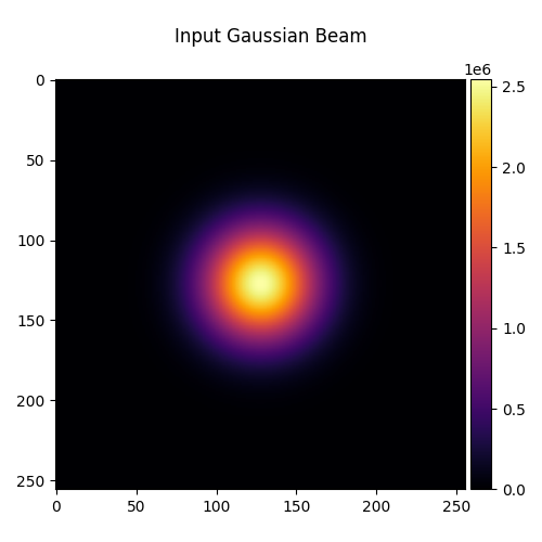
Input Field

We use a Gaussian beam as the input.

input_field = Field(gaussian(shape, waist_radius=waist_radius)).to(device)
visualize_tensor(input_field.intensity(), title="Input Gaussian Beam")

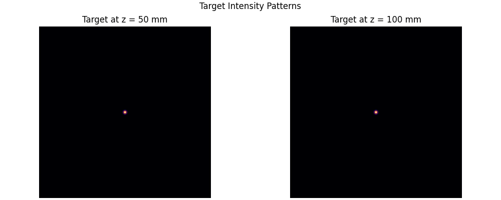
Target Patterns

At each focal plane, we want a focused Gaussian spot. The target spot size is determined by the diffraction limit.

# Target: Gaussian spots at each focal plane
target_waist = 30e-6  # Target spot size (m)

target_1 = Field(gaussian(shape, waist_radius=target_waist), z=focal_plane_1).to(device)
target_2 = Field(gaussian(shape, waist_radius=target_waist), z=focal_plane_2).to(device)

fig, (ax1, ax2) = plt.subplots(1, 2, figsize=(10, 4), constrained_layout=True)

ax1.imshow(target_1.intensity().cpu(), cmap="inferno")
ax1.set_title(f"Target at z = {focal_plane_1 * 1e3:.0f} mm")
ax1.axis("off")

ax2.imshow(target_2.intensity().cpu(), cmap="inferno")
ax2.set_title(f"Target at z = {focal_plane_2 * 1e3:.0f} mm")
ax2.axis("off")

plt.suptitle("Target Intensity Patterns", fontsize=12)
plt.show()

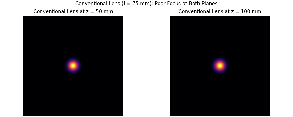
Conventional Lens Comparison

First, let’s see what happens with a conventional lens focused at the midpoint. It cannot achieve good focus at both planes.

midpoint_focus = (focal_plane_1 + focal_plane_2) / 2
conventional_lens = Lens(shape, midpoint_focus, z=0).to(device)

# Propagate through conventional lens
field_after_lens = conventional_lens(input_field)
output_1_conv = field_after_lens.propagate_to_z(focal_plane_1)
output_2_conv = field_after_lens.propagate_to_z(focal_plane_2)

fig, (ax1, ax2) = plt.subplots(1, 2, figsize=(10, 4), constrained_layout=True)

ax1.imshow(output_1_conv.intensity().cpu(), cmap="inferno")
ax1.set_title(f"Conventional Lens at z = {focal_plane_1 * 1e3:.0f} mm")
ax1.axis("off")

ax2.imshow(output_2_conv.intensity().cpu(), cmap="inferno")
ax2.set_title(f"Conventional Lens at z = {focal_plane_2 * 1e3:.0f} mm")
ax2.axis("off")

plt.suptitle(f"Conventional Lens (f = {midpoint_focus * 1e3:.0f} mm): Poor Focus at Both Planes", fontsize=12)
plt.show()

Diffractive Multi-Focal Element

We design a phase-only diffractive element that can focus at both planes.

# Initialize with zeros (will be optimized)
phase_modulator = PhaseModulator(Parameter(torch.zeros(shape, shape)), z=0).to(device)

Training Loop

We optimize the phase pattern to maximize the overlap with target patterns at both focal planes.

optimizer = torch.optim.Adam(phase_modulator.parameters(), lr=0.1)
num_iterations = 100

losses = []
losses_plane1 = []
losses_plane2 = []

for iteration in range(num_iterations):
    optimizer.zero_grad()

    # Apply phase modulator
    field_after_mod = phase_modulator(input_field)

    # Propagate to both focal planes
    output_1 = field_after_mod.propagate_to_z(focal_plane_1)
    output_2 = field_after_mod.propagate_to_z(focal_plane_2)

    # Loss: maximize overlap with targets at both planes (equal weight)
    overlap_1 = output_1.inner(target_1).abs().square()
    overlap_2 = output_2.inner(target_2).abs().square()

    loss_1 = 1 - overlap_1
    loss_2 = 1 - overlap_2
    loss = loss_1 + loss_2  # Equal weighting

    loss.backward()
    optimizer.step()

    losses.append(loss.item())
    losses_plane1.append(loss_1.item())
    losses_plane2.append(loss_2.item())

    if iteration % 50 == 0:
        print(
            f"Iteration {iteration}: Total Loss = {loss.item():.4f}, "
            f"Plane 1 = {loss_1.item():.4f}, Plane 2 = {loss_2.item():.4f}"
        )

Iteration 0: Total Loss = 1.9715, Plane 1 = 0.9857, Plane 2 = 0.9858
Iteration 50: Total Loss = 0.9989, Plane 1 = 0.4859, Plane 2 = 0.5130

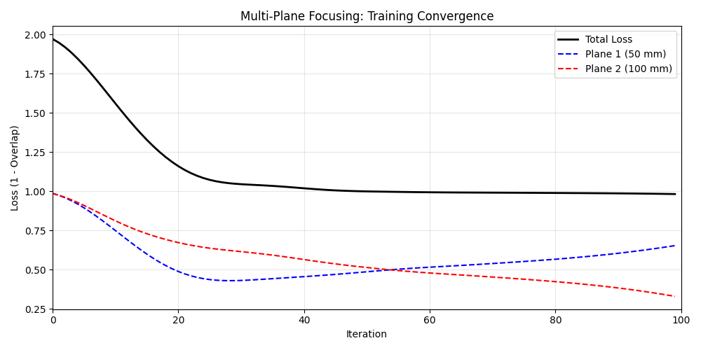
Training Convergence

We plot the loss curves for both focal planes.

fig, ax = plt.subplots(figsize=(10, 5))
ax.plot(losses, "k-", linewidth=2, label="Total Loss")
ax.plot(losses_plane1, "b--", linewidth=1.5, label=f"Plane 1 ({focal_plane_1 * 1e3:.0f} mm)")
ax.plot(losses_plane2, "r--", linewidth=1.5, label=f"Plane 2 ({focal_plane_2 * 1e3:.0f} mm)")
ax.set_xlabel("Iteration")
ax.set_ylabel("Loss (1 - Overlap)")
ax.set_title("Multi-Plane Focusing: Training Convergence")
ax.legend()
ax.grid(True, alpha=0.3)
ax.set_xlim(0, num_iterations)
plt.tight_layout()
plt.show()

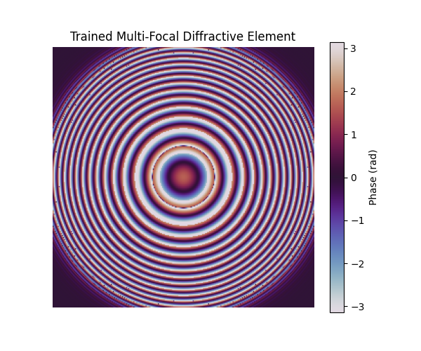
Trained Phase Pattern

The optimized phase pattern is a complex diffractive structure that splits and focuses light at multiple planes.

trained_phase = phase_modulator.phase.data.cpu()

fig, ax = plt.subplots(figsize=(6, 5))
im = ax.imshow(trained_phase, cmap="twilight", vmin=-torch.pi, vmax=torch.pi)
ax.set_title("Trained Multi-Focal Diffractive Element")
ax.axis("off")
fig.colorbar(im, ax=ax, label="Phase (rad)")
plt.show()

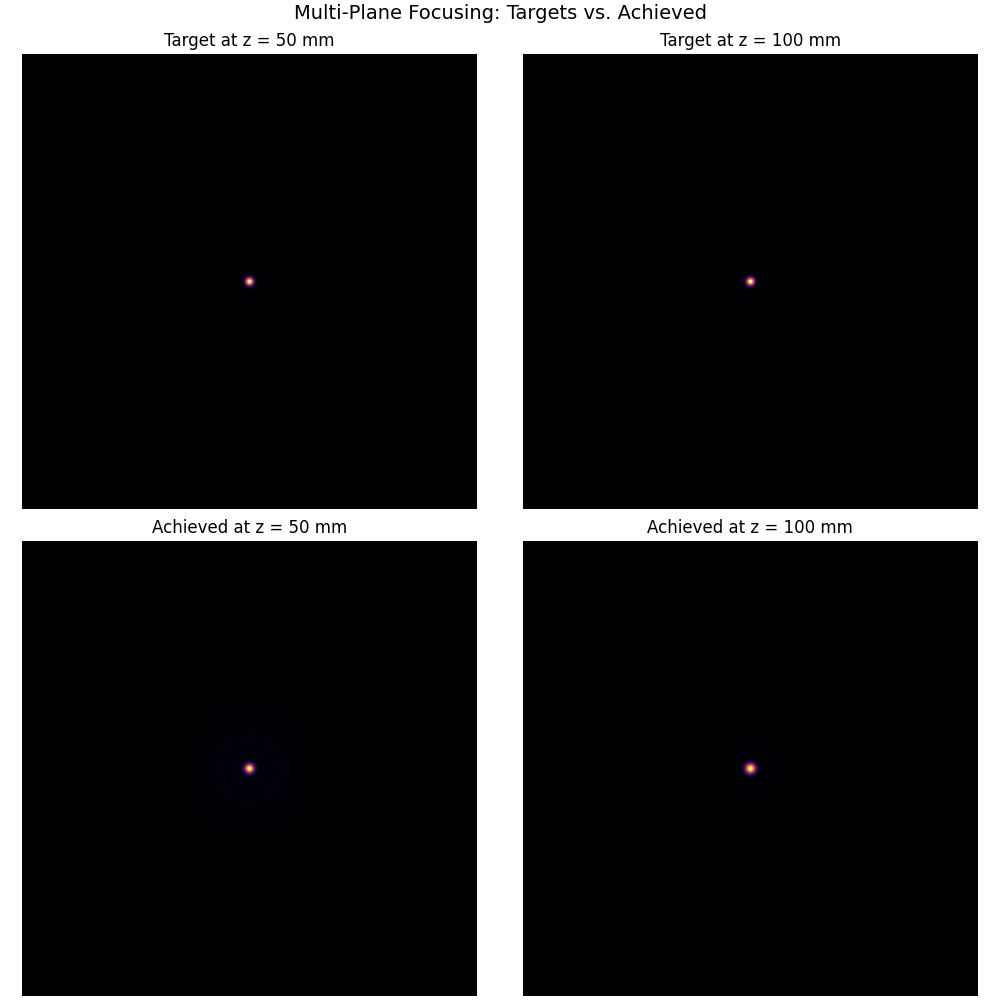
Results: Multi-Plane Focus

The trained element achieves good focus at both target planes.

# Final outputs (detach from computation graph for visualization)
with torch.no_grad():
    field_after_mod = phase_modulator(input_field)
    output_1_trained = field_after_mod.propagate_to_z(focal_plane_1)
    output_2_trained = field_after_mod.propagate_to_z(focal_plane_2)

fig, axes = plt.subplots(2, 2, figsize=(10, 10), constrained_layout=True)

# Targets
axes[0, 0].imshow(target_1.intensity().cpu(), cmap="inferno")
axes[0, 0].set_title(f"Target at z = {focal_plane_1 * 1e3:.0f} mm")
axes[0, 0].axis("off")

axes[0, 1].imshow(target_2.intensity().cpu(), cmap="inferno")
axes[0, 1].set_title(f"Target at z = {focal_plane_2 * 1e3:.0f} mm")
axes[0, 1].axis("off")

# Achieved
axes[1, 0].imshow(output_1_trained.intensity().cpu(), cmap="inferno")
axes[1, 0].set_title(f"Achieved at z = {focal_plane_1 * 1e3:.0f} mm")
axes[1, 0].axis("off")

axes[1, 1].imshow(output_2_trained.intensity().cpu(), cmap="inferno")
axes[1, 1].set_title(f"Achieved at z = {focal_plane_2 * 1e3:.0f} mm")
axes[1, 1].axis("off")

plt.suptitle("Multi-Plane Focusing: Targets vs. Achieved", fontsize=14)
plt.show()

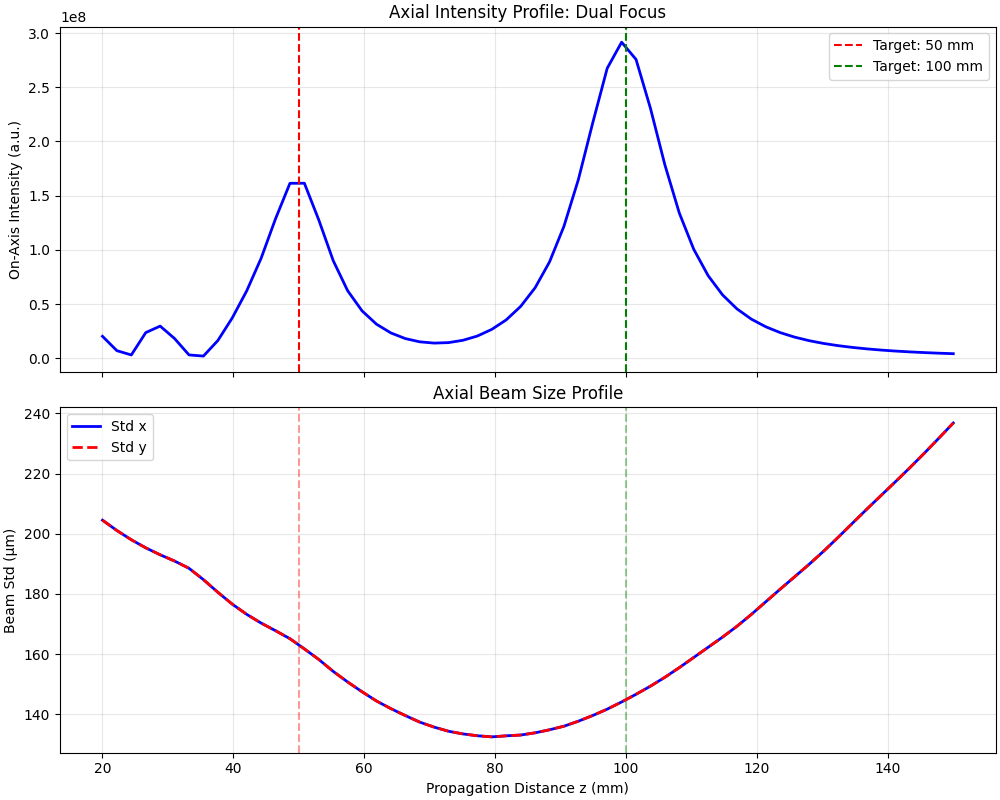
Axial Intensity Profile

We examine the intensity distribution along the optical axis to see the dual focusing behavior. The beam standard deviation (spot size) is also plotted to show how the beam converges and diverges at each focus.

num_z = 60
z_range = torch.linspace(20e-3, 150e-3, num_z)
on_axis_intensity = []
std_x = []
std_y = []
center = shape // 2

with torch.no_grad():
    for z in z_range:
        output = field_after_mod.propagate_to_z(z.item())
        intensity = output.intensity().cpu()
        on_axis_intensity.append(intensity[center, center].item())
        std = output.std().cpu()
        std_x.append(std[0].item())
        std_y.append(std[1].item())

fig, (ax1, ax2) = plt.subplots(2, 1, figsize=(10, 8), sharex=True, constrained_layout=True)

ax1.plot(z_range * 1e3, on_axis_intensity, "b-", linewidth=2)
ax1.axvline(focal_plane_1 * 1e3, color="r", linestyle="--", label=f"Target: {focal_plane_1 * 1e3:.0f} mm")
ax1.axvline(focal_plane_2 * 1e3, color="g", linestyle="--", label=f"Target: {focal_plane_2 * 1e3:.0f} mm")
ax1.set_ylabel("On-Axis Intensity (a.u.)")
ax1.set_title("Axial Intensity Profile: Dual Focus")
ax1.legend()
ax1.grid(True, alpha=0.3)

ax2.plot(z_range * 1e3, [s * 1e6 for s in std_x], "b-", linewidth=2, label="Std x")
ax2.plot(z_range * 1e3, [s * 1e6 for s in std_y], "r--", linewidth=2, label="Std y")
ax2.axvline(focal_plane_1 * 1e3, color="r", linestyle="--", alpha=0.4)
ax2.axvline(focal_plane_2 * 1e3, color="g", linestyle="--", alpha=0.4)
ax2.set_xlabel("Propagation Distance z (mm)")
ax2.set_ylabel("Beam Std (µm)")
ax2.set_title("Axial Beam Size Profile")
ax2.legend()
ax2.grid(True, alpha=0.3)

plt.show()

Comparison with Bifocal Lens

Our trained element is similar in function to a bifocal lens, but with arbitrary focal lengths and ratios achievable through optimization.

print("\nFinal Performance:")
print(f"  Overlap at z = {focal_plane_1 * 1e3:.0f} mm: {1 - losses_plane1[-1]:.3f}")
print(f"  Overlap at z = {focal_plane_2 * 1e3:.0f} mm: {1 - losses_plane2[-1]:.3f}")
print(f"  Total efficiency: {(2 - losses[-1]) / 2:.3f}")

Final Performance:
  Overlap at z = 50 mm: 0.347
  Overlap at z = 100 mm: 0.671
  Total efficiency: 0.509