Lens Focusing

Demonstrates how a thin lens focuses a collimated Gaussian beam to its focal plane. Shows the propagation through focus and how beam size varies with propagation distance for different focal lengths.

import matplotlib.pyplot as plt
import torch

import torchoptics
from torchoptics import Field, System, visualize_tensor
from torchoptics.elements import Lens
from torchoptics.profiles import gaussian

Simulation Parameters

A lens with focal length \(f\) focuses a collimated Gaussian beam to its back focal plane. The focused spot size is:

\[w_f = \frac{\lambda f}{\pi w_0}\]

where \(w_0\) is the input beam waist.

shape = 512  # Grid size
spacing = 10e-6  # Grid spacing (m)
wavelength = 632.8e-9  # HeNe laser wavelength (m)

focal_length = 100e-3  # Lens focal length (m)
beam_waist = 1e-3  # Input beam waist (m)

w_focus = wavelength * focal_length / (torch.pi * beam_waist)

torchoptics.set_default_spacing(spacing)
torchoptics.set_default_wavelength(wavelength)

device = "cuda" if torch.cuda.is_available() else "cpu"

print(f"Focal length:         {focal_length * 1e3:.0f} mm")
print(f"Input beam waist:     {beam_waist * 1e3:.1f} mm")
print(f"Predicted spot size:  {w_focus * 1e6:.1f} µm")

Focal length:         100 mm
Input beam waist:     1.0 mm
Predicted spot size:  20.1 µm

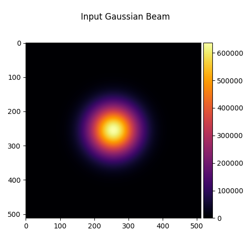
Input Field: Gaussian Beam

A collimated Gaussian beam is created at the lens plane.

profile = gaussian(shape, waist_radius=beam_waist)
input_field = Field(profile).to(device)

visualize_tensor(input_field.intensity(), title="Input Gaussian Beam")

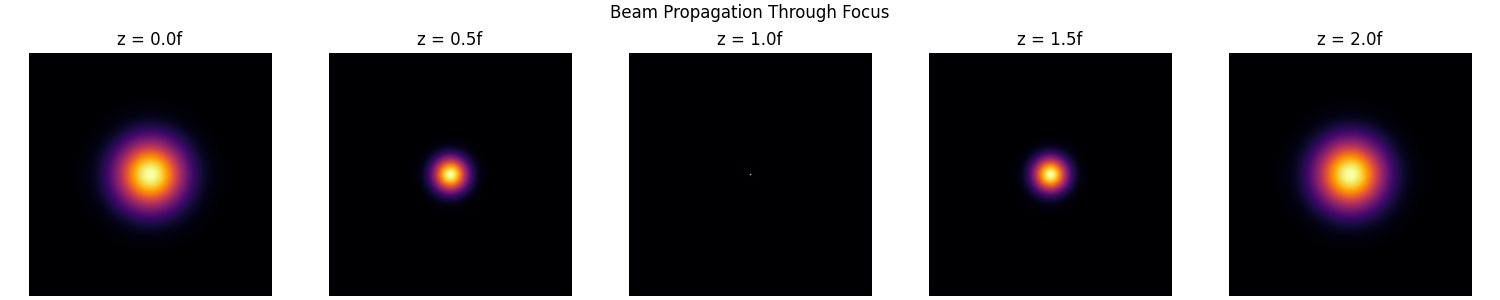
Propagation Through Focus

We propagate the beam through a single lens and sample the intensity at five planes from the lens to twice the focal length.

system = System(Lens(shape, focal_length=focal_length, z=0)).to(device)
after_lens = system(input_field)

z_positions = torch.linspace(0, 2 * focal_length, 5)

fig, axes = plt.subplots(1, 5, figsize=(15, 3), constrained_layout=True)

for ax, z in zip(axes, z_positions):
    intensity = after_lens.propagate_to_z(z).intensity().cpu()
    ax.imshow(intensity, cmap="inferno")
    ax.set_title(f"z = {z / focal_length:.1f}f")
    ax.axis("off")

plt.suptitle("Beam Propagation Through Focus")
plt.show()

Beam Size vs. Propagation Distance

Field.std() returns the intensity-weighted standard deviation \(\sigma = w/2\) for a Gaussian, where \(w\) is the 1/e² beam radius. Multiplying by 2 gives the beam waist directly, which can be compared to the theoretical prediction \(w_f = \lambda f / \pi w_0\).

focal_lengths = [100e-3, 150e-3, 200e-3]  # Focal lengths to compare (m)

fig, ax = plt.subplots(figsize=(8, 4), constrained_layout=True)

z_positions = torch.linspace(0, 300e-3, 51)

for f in focal_lengths:
    after_lens_f = System(Lens(shape, focal_length=f, z=0)).to(device)(input_field)
    waists_x = [2 * after_lens_f.propagate_to_z(z).std().cpu()[1] for z in z_positions]
    w_theory = wavelength * f / (torch.pi * beam_waist)
    ax.plot(z_positions * 1e3, torch.stack(waists_x) * 1e6, label=f"f = {f * 1e3:.0f} mm")
    ax.axvline(f * 1e3, color="gray", linestyle=":", linewidth=0.8)
    ax.annotate(
        f"{w_theory * 1e6:.1f} µm",
        xy=(f * 1e3, w_theory * 1e6),
        xytext=(4, 4),
        textcoords="offset points",
        fontsize=7,
        color="gray",
    )

ax.set_xlim(0, None)
ax.set_xlabel("z (mm)")
ax.set_ylabel("Beam waist (µm)")
ax.set_title("Beam Size vs. Propagation Distance")
ax.legend()
plt.show()

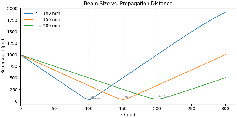
A lens performs a spatial Fourier transform, mapping each input spatial frequency to a unique position at the focal plane. Shorter focal lengths produce tighter foci but also diverge more rapidly beyond the focal plane.