Polarized Field

Simulates how a polarized Gaussian beam responds to polarizers and waveplates.

import matplotlib.pyplot as plt
import torch

import torchoptics
from torchoptics import Field
from torchoptics.elements import HalfWaveplate, LinearPolarizer, QuarterWaveplate
from torchoptics.profiles import gaussian

Simulation Parameters

Define the grid size and set default optical properties.

shape = 100  # Grid size (number of points per dimension)
spacing = 10e-6  # Grid spacing (m)
wavelength = 700e-9  # Wavelength (m)
beam_waist = 250e-6  # Beam waist radius (m)
extent_mm = (shape - 1) * spacing / 2 * 1e3
x_coords = torch.linspace(-extent_mm, extent_mm, shape)

# Configure torchoptics defaults
torchoptics.set_default_spacing(spacing)
torchoptics.set_default_wavelength(wavelength)

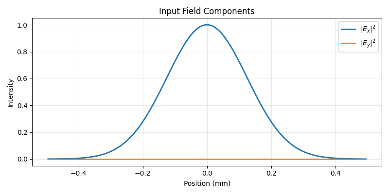
Initializing a Polarized Field

A polarized field has shape (3, H, W); the three components are \(E_x\), \(E_y\), \(E_z\). Here we initialize a Gaussian beam with pure \(x\)-linear polarization (horizontal).

field_profile = gaussian(shape, waist_radius=beam_waist).real
field_data = torch.zeros(3, shape, shape, dtype=field_profile.dtype)
field_data[0] = field_profile
field = Field(field_data).normalize()

# Plot the input field components along the center row.
center_row = shape // 2
input_profile = field.data[0].abs().square().cpu()[center_row, :]
input_profile_max = input_profile.max()
input_ex = input_profile / input_profile_max
input_ey = field.data[1].abs().square().cpu()[center_row, :] / input_profile_max

fig, ax = plt.subplots(figsize=(8, 4))
ax.plot(x_coords, input_ex, linewidth=2, label=r"$|E_x|^2$")
ax.plot(x_coords, input_ey, linewidth=2, label=r"$|E_y|^2$")
ax.set_xlabel("Position (mm)")
ax.set_ylabel("Intensity")
ax.set_title("Input Field Components")
ax.legend()
ax.grid(True, alpha=0.3)
plt.tight_layout()
plt.show()

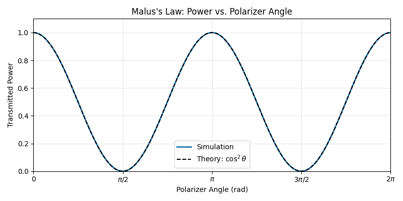
Malus’s Law: Power Transmission Through a Rotating Polarizer

We apply linear polarizers at different angles ranging from 0 to \(2\pi\) radians. Malus’s law states that the transmitted power follows:

\[P = P_0 \cos^2(\theta)\]

where \(P_0\) is the initial power, and \(\theta\) is the angle between the initial polarization and the polarizer’s axis.

angles = torch.linspace(0, 2 * torch.pi, 400)
field_power = torch.tensor(
    [LinearPolarizer(shape, theta=float(theta))(field).power().sum().item() for theta in angles]
)
theory = torch.cos(angles) ** 2

fig, ax = plt.subplots(figsize=(8, 4))
ax.plot(angles, field_power, linewidth=2, label="Simulation")
ax.plot(angles, theory, "k--", linewidth=1.5, label=r"Theory: $\cos^2\theta$")
ax.set_xlim(float(angles.min()), float(angles.max()))
ax.set_ylim(0, 1.1)
ax.set_xticks(
    [0.0, float(torch.pi / 2), float(torch.pi), float(3 * torch.pi / 2), float(2 * torch.pi)],
    ["0", r"$\pi/2$", r"$\pi$", r"$3\pi/2$", r"$2\pi$"],
)
ax.set_xlabel("Polarizer Angle (rad)")
ax.set_ylabel("Transmitted Power")
ax.set_title("Malus's Law: Power vs. Polarizer Angle")
ax.legend()
ax.grid(True, alpha=0.3)
plt.tight_layout()
plt.show()

Sequential Polarizers and Projection Effects

Applying two polarizers in sequence highlights an important property of polarization:

• A 90° polarizer alone completely blocks light polarized along 0°.

• However, inserting an intermediate 45° polarizer allows some light to pass through.

• The second polarizer (90°) then transmits part of this newly polarized light.

The first polarizer projects the field onto a new axis, enabling partial transmission through the second polarizer.

polarizer_0 = LinearPolarizer(shape, theta=0)
polarizer_45 = LinearPolarizer(shape, theta=torch.pi / 4)
polarizer_90 = LinearPolarizer(shape, theta=torch.pi / 2)

after_0 = polarizer_0(field)
after_45 = polarizer_45(field)
after_90 = polarizer_90(field)
after_45_90 = polarizer_90(after_45)

stage_labels = ["Input", "0°", "45°", "90°", "45° → 90°"]
stage_powers = [
    field.power().sum().item(),
    after_0.power().sum().item(),
    after_45.power().sum().item(),
    after_90.power().sum().item(),
    after_45_90.power().sum().item(),
]

print("Sequential Polarizer Experiment")
for label, power in zip(stage_labels, stage_powers):
    print(f"  {label:<10}: {power:.3f}")

Sequential Polarizer Experiment
  Input     : 1.000
  0°        : 1.000
  45°       : 0.500
  90°       : 0.000
  45° → 90° : 0.250

Quarter- and Half-Waveplates

A quarter-waveplate with its fast axis at \(45°\) converts linear polarization into circular polarization. A half-waveplate at the same angle rotates the polarization axis by \(90°\).

qwp_45 = QuarterWaveplate(shape, theta=torch.pi / 4)
hwp_45 = HalfWaveplate(shape, theta=torch.pi / 4)

after_qwp = qwp_45(field)
after_hwp = hwp_45(field)

for label, f, theory in [
    ("Quarter-waveplate at 45° (linear → circular)", after_qwp, "S1= 0.000  S2= 0.000  S3=+1.000"),
    ("Half-waveplate at 45°   (horizontal → vertical)", after_hwp, "S1=-1.000  S2= 0.000  S3= 0.000"),
]:
    ex, ey = f.data[0], f.data[1]
    i = ex.abs().square() + ey.abs().square()
    s1 = ((ex.abs().square() - ey.abs().square()) / (i + 1e-12)).mean().item()
    s2 = (2 * (ex * ey.conj()).real / (i + 1e-12)).mean().item()
    s3 = (2 * (ex * ey.conj()).imag / (i + 1e-12)).mean().item()
    print(f"\n{label}:")
    print(f"  S1={s1:+.3f}  S2={s2:+.3f}  S3={s3:+.3f}  (theory: {theory})")

Quarter-waveplate at 45° (linear → circular):
  S1=+0.000  S2=+0.000  S3=+1.000  (theory: S1= 0.000  S2= 0.000  S3=+1.000)

Half-waveplate at 45°   (horizontal → vertical):
  S1=-1.000  S2=+0.000  S3=+0.000  (theory: S1=-1.000  S2= 0.000  S3= 0.000)

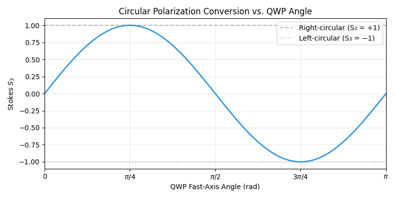
Waveplate Rotation Sweep

Sweeping the quarter-waveplate axis angle tracks the circular polarization content through the Stokes parameter \(S_3\).

waveplate_angles = torch.linspace(0, torch.pi, 200)
s3_values = []

for theta in waveplate_angles:
    qwp = QuarterWaveplate(shape, theta=float(theta))
    out = qwp(field)
    ex_out = out.data[0]
    ey_out = out.data[1]
    intensity = ex_out.abs().square() + ey_out.abs().square()
    s3_values.append((2 * (ex_out * ey_out.conj()).imag / (intensity + 1e-12)).mean().item())

fig, ax = plt.subplots(figsize=(8, 4))
ax.plot(waveplate_angles, s3_values, color="#3498db", linewidth=2)
ax.axhline(1.0, color="gray", linestyle="--", alpha=0.5, label="Right-circular (S₃ = +1)")
ax.axhline(-1.0, color="gray", linestyle=":", alpha=0.5, label="Left-circular (S₃ = −1)")
ax.set_xlabel("QWP Fast-Axis Angle (rad)")
ax.set_ylabel(r"Stokes $S_3$")
ax.set_title("Circular Polarization Conversion vs. QWP Angle")
ax.set_xticks([0.0, float(torch.pi / 4), float(torch.pi / 2), float(3 * torch.pi / 4), float(torch.pi)])
ax.set_xticklabels(["0", r"$\pi/4$", r"$\pi/2$", r"$3\pi/4$", r"$\pi$"])
ax.set_xlim(0, float(torch.pi))
ax.set_ylim(-1.1, 1.1)
ax.legend()
ax.grid(True, alpha=0.3)
plt.tight_layout()
plt.show()