
Note
Go to the end to download the full example code.
Spatial Coherence#
Simulates partially coherent Gaussian beams using the Gaussian-Schell model (GSM). Spatial coherence describes the correlation of a field at two different spatial points. In the GSM, the coherence width \(\sigma_c\) controls how correlated the field is across the beam profile:
When \(\sigma_c \gg w_0\) the field is nearly fully coherent; when \(\sigma_c \ll w_0\) it is highly incoherent and diverges rapidly upon propagation.
import torch

import torchoptics
from torchoptics import SpatialCoherence
from torchoptics.profiles import gaussian_schell_model as gsm
Simulation Parameters#
We compare two beams with identical intensity profiles but different coherence widths. The coherence width relative to the beam waist determines the divergence behavior during propagation.
shape = 30  # Grid size (number of points per dimension)
spacing = 10e-6  # Grid spacing (m)
wavelength = 700e-9  # Wavelength (m)
waist_radius = 40e-6  # Waist radius of the Gaussian beam (m)

# Define coherence widths
low_coherence_width = 10e-6  # Low spatial coherence (m)
high_coherence_width = 1e-3  # High spatial coherence (m)

# Determine computation device
device = "cuda" if torch.cuda.is_available() else "cpu"

# Configure torchoptics defaults
torchoptics.set_default_spacing(spacing)
torchoptics.set_default_wavelength(wavelength)

print(f"Beam waist: {waist_radius * 1e6:.0f} µm")
low_ratio = low_coherence_width / waist_radius
print(f"Low coherence width: {low_coherence_width * 1e6:.0f} µm (σ_c/w₀ = {low_ratio:.2f})")
high_ratio = high_coherence_width / waist_radius
print(f"High coherence width: {high_coherence_width * 1e3:.1f} mm (σ_c/w₀ = {high_ratio:.0f})")
Beam waist: 40 µm
Low coherence width: 10 µm (σ_c/w₀ = 0.25)
High coherence width: 1.0 mm (σ_c/w₀ = 25)
Coherence Matrices#
The Gaussian-Schell model generates a mutual coherence matrix that encodes
both the intensity profile and the spatial correlations. We initialize two
SpatialCoherence objects representing low- and
high-coherence beams.
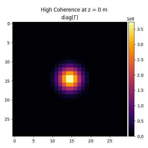
Propagation Comparison#
Low-coherence fields spread rapidly and lose structure, while high-coherence fields maintain their spatial distribution over longer distances, analogous to how a laser beam (high coherence) stays collimated while a thermal source (low coherence) diverges quickly.
propagation_distances = [0, 0.01, 0.02]

for z in propagation_distances:
    low_spatial_coherence.propagate_to_z(z).visualize(title=f"Low Coherence at z = {z} m", vmin=0)
    high_spatial_coherence.propagate_to_z(z).visualize(title=f"High Coherence at z = {z} m", vmin=0)


Total running time of the script: (0 minutes 1.352 seconds)