Chromatic Aberration of a Dispersive Lens

Simulates the longitudinal chromatic aberration of a plano-convex BK7 glass lens, where wavelength-dependent dispersion causes each colour to focus at a different distance along the optical axis. The PolychromaticPhaseModulator stores the physical thickness profile and a dispersive refractive-index function, automatically computing the correct wavelength-dependent phase without any changes to the optical system between wavelengths.

For a plano-convex lens with radius of curvature \(R\) and refractive index \(n(\lambda)\), the paraxial focal length is:

\[f(\lambda) = \frac{R}{n(\lambda) - 1}\]

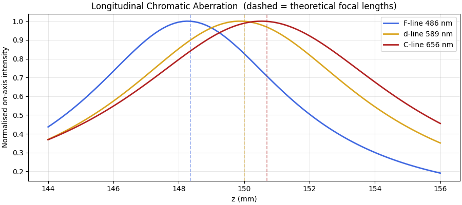
Because glass has higher refractive index at shorter wavelengths (normal dispersion), blue light focuses closer to the lens than red. The longitudinal chromatic aberration (LCA) is approximately \(\Delta f \approx f_d / V_d\), where \(V_d = (n_d - 1)\,/\,(n_F - n_C)\) is the Abbe number.

import matplotlib.pyplot as plt
import torch

import torchoptics
from torchoptics import Field, System
from torchoptics.elements import PolychromaticPhaseModulator
from torchoptics.profiles import gaussian
from torchoptics.profiles._profile_meshgrid import profile_meshgrid

Simulation Parameters

Three standard Fraunhofer spectral lines are simulated: F (blue, 486 nm), d (yellow, 589 nm), and C (red, 656 nm). BK7 dispersion is modelled by a two-term Cauchy equation \(n(\lambda) = A + B/\lambda^2\).

shape = 512
spacing = 10e-6  # 10 µm grid spacing — large enough that the 1 mm beam
# decays to < 0.2 % amplitude at the boundary
waist_radius = 1e-3  # 1 mm Gaussian beam waist

# BK7 glass Cauchy coefficients
A_cauchy = 1.5044
B_cauchy = 4.24e-15  # m²


def n_bk7(wavelength):
    """Two-term Cauchy dispersion model for BK7 glass."""
    return A_cauchy + B_cauchy / wavelength**2


# Fraunhofer spectral lines
wavelengths = [486.1e-9, 589.3e-9, 656.3e-9]  # F, d, C lines (m)
colors = ["royalblue", "goldenrod", "firebrick"]
labels = ["F-line 486 nm", "d-line 589 nm", "C-line 656 nm"]

# Lens geometry: plano-convex, designed for f_d = 150 mm at the d-line
n_d = n_bk7(589.3e-9)
focal_d = 150e-3  # design focal length at d-line (m)
R = focal_d * (n_d - 1)  # radius of curvature (m)

# Abbe number and theoretical focal lengths
n_F, n_C = n_bk7(486.1e-9), n_bk7(656.3e-9)
V_abbe = (n_d - 1) / (n_F - n_C)
focal_theory = [R / (n_bk7(wl) - 1) for wl in wavelengths]
lca_theory = focal_theory[2] - focal_theory[0]

torchoptics.set_default_spacing(spacing)
device = "cuda" if torch.cuda.is_available() else "cpu"

print(f"BK7 refractive indices:  nF = {n_F:.4f},  nd = {n_d:.4f},  nC = {n_C:.4f}")
print(f"Abbe number:             Vd = {V_abbe:.1f}")
print(f"Radius of curvature:     R  = {R * 1e3:.2f} mm")
print(f"Theoretical LCA:         Δf = f_d / Vd = {lca_theory * 1e3:.2f} mm")

BK7 refractive indices:  nF = 1.5223,  nd = 1.5166,  nC = 1.5142
Abbe number:             Vd = 63.8
Radius of curvature:     R  = 77.49 mm
Theoretical LCA:         Δf = f_d / Vd = 2.34 mm

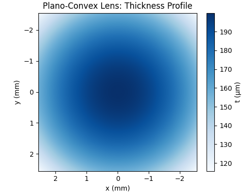
Lens Thickness Profile

The plano-convex lens has a quadratic thickness profile. The same physical thickness produces a different optical path length at every wavelength, giving a wavelength-dependent focal length.

x, y = profile_meshgrid(shape, spacing, None)
r_squared = x**2 + y**2

t_center = 200e-6  # on-axis centre thickness (m)
thickness = (t_center - r_squared / (2 * R)).clamp(min=0)

lim_mm = float(x[0, -1].item() * 1e3)
fig, ax = plt.subplots(figsize=(5, 4), constrained_layout=True)
im = ax.imshow(
    thickness.numpy() * 1e6,
    cmap="Blues",
    extent=(-lim_mm, lim_mm, -lim_mm, lim_mm),
)
ax.set_title("Plano-Convex Lens: Thickness Profile")
ax.set_xlabel("x (mm)")
ax.set_ylabel("y (mm)")
fig.colorbar(im, ax=ax, label="t (µm)")
plt.show()

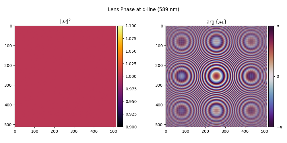
Polychromatic Phase Modulator

The PolychromaticPhaseModulator applies

\[\mathcal{M}(x, y) = \exp\!\left(i\,\frac{2\pi}{\lambda} \bigl[n(\lambda) - 1\bigr]\, t(x, y)\right)\]

at the field’s own wavelength, so the same element correctly handles every colour without modification. Below we visualise the phase at the d-line.

lens = PolychromaticPhaseModulator(thickness, n=n_bk7)
system = System(lens).to(device)

system[0].visualize(wavelength=589.3e-9, title="Lens Phase at d-line (589 nm)")

Input Fields

One collimated Gaussian field per wavelength; all share the same spatial profile and propagate through the same optical system.

gaussian_profile = gaussian(shape, waist_radius)
fields = [Field(gaussian_profile, wavelength=wl).to(device) for wl in wavelengths]

On-Axis Intensity vs. Propagation Distance

After the lens, each wavelength focuses at a different \(z\). Scanning the on-axis intensity reveals three distinct peaks. Dashed lines mark the theoretical focal lengths from the lens-maker’s equation.

z_scan = torch.linspace(144e-3, 156e-3, 100)
cx = shape // 2

on_axis = []
for field in fields:
    row = [system.measure_at_z(field, z.item()).intensity()[cx, cx].item() for z in z_scan]
    on_axis.append(torch.tensor(row))

fig, ax = plt.subplots(figsize=(9, 4), constrained_layout=True)
for intensity, lbl, clr, f_th in zip(on_axis, labels, colors, focal_theory):
    ax.plot(z_scan * 1e3, intensity / intensity.max(), color=clr, linewidth=2, label=lbl)
    ax.axvline(f_th * 1e3, color=clr, linestyle="--", alpha=0.5, linewidth=1.2)

ax.set_xlabel("z (mm)")
ax.set_ylabel("Normalised on-axis intensity")
ax.set_title("Longitudinal Chromatic Aberration  (dashed = theoretical focal lengths)")
ax.legend()
ax.grid(True, alpha=0.3)
plt.show()