Zernike Aberrations

Visualizes common optical aberrations using Zernike polynomials and shows how each aberration degrades the point spread function (PSF) of a lens. Zernike polynomials form a natural basis for describing wavefront errors over a circular pupil and are widely used in adaptive optics, ophthalmology, and optical testing.

import matplotlib.pyplot as plt
import torch

import torchoptics
from torchoptics import Field, System, visualize_tensor
from torchoptics.elements import Modulator
from torchoptics.profiles import circle, lens_phase, zernike

Simulation Parameters

shape = 500  # Grid size (number of points per dimension)
spacing = 10e-6  # Grid spacing (m)
wavelength = 500e-9  # Wavelength (m)

focal_length = 0.5  # Lens focal length (m)
aperture_radius = 1.5e-3  # Lens aperture radius (m)
d_o = 1.0  # Object distance (m)
d_i = 1.0  # Image distance (m), satisfies 1/f = 1/d_o + 1/d_i

aberration_strength = 4 * torch.pi  # Peak-to-valley wavefront error (~2 waves)

# Configure torchoptics defaults
torchoptics.set_default_spacing(spacing)
torchoptics.set_default_wavelength(wavelength)

# Select computation device
device = "cuda" if torch.cuda.is_available() else "cpu"

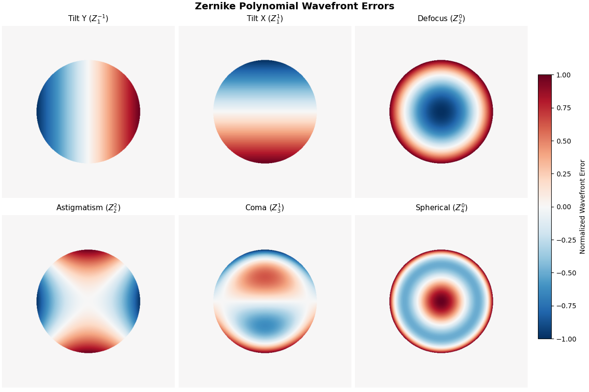
Zernike Polynomial Gallery

The most common aberration types and their Zernike polynomial indices:

aberrations = [
    (1, -1, "Tilt Y"),
    (1, 1, "Tilt X"),
    (2, 0, "Defocus"),
    (2, 2, "Astigmatism"),
    (3, 1, "Coma"),
    (4, 0, "Spherical"),
]

fig, axes = plt.subplots(2, 3, figsize=(12, 8), constrained_layout=True)
fig.suptitle("Zernike Polynomial Wavefront Errors", fontsize=14, fontweight="bold")

for ax, (n, m, name) in zip(axes.flat, aberrations):
    z_poly = zernike(shape, n, m, aperture_radius)
    ax.imshow(z_poly, cmap="RdBu_r", vmin=-1, vmax=1)
    ax.set_title(rf"{name} ($Z_{{{n}}}^{{{m}}}$)", fontsize=11)
    ax.axis("off")

fig.colorbar(axes.flat[0].images[0], ax=axes, label="Normalized Wavefront Error", shrink=0.72, pad=0.02)
plt.show()

Point Source Input

We create a delta-function point source to measure the PSF.

point_source_data = torch.zeros(shape, shape)
point_source_data[shape // 2, shape // 2] = 1.0
point_source = Field(point_source_data).to(device)

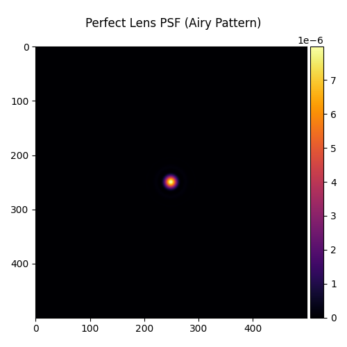
PSF: Perfect vs. Aberrated Lens

We compare the PSF of a perfect lens with lenses affected by each Zernike aberration. The aberrated wavefront is:

\[W(x, y) = \phi_{\text{lens}}(x, y) + \alpha \, Z_n^m(x, y)\]

where \(\alpha\) controls the aberration strength.

# Build perfect lens profile
phase = lens_phase(shape, focal_length)
pupil = circle(shape, aperture_radius)

# Perfect PSF
perfect_lens = Modulator(pupil * torch.exp(1j * phase), z=d_o).to(device)
perfect_psf = System(perfect_lens).measure_at_z(point_source, z=d_o + d_i)
visualize_tensor(perfect_psf.intensity(), title="Perfect Lens PSF (Airy Pattern)")

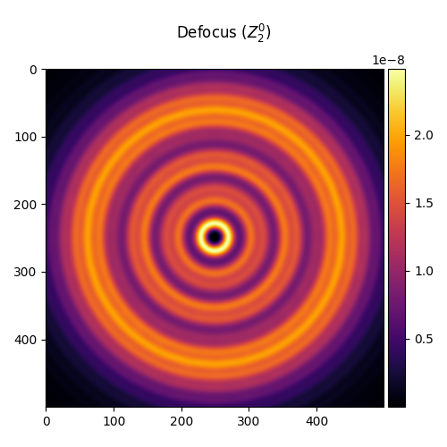
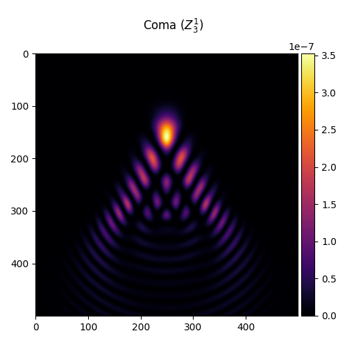
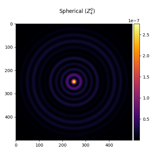
Aberrated PSFs

Each aberration distorts the PSF in a distinct way: coma produces a comet-like tail, astigmatism elongates the spot, and spherical aberration creates a diffuse halo.

aberrations_for_psf = [
    (2, 0, "Defocus"),
    (2, 2, "Astigmatism"),
    (3, 1, "Coma"),
    (4, 0, "Spherical"),
]

for n, m, name in aberrations_for_psf:
    # Add wavefront error to lens phase
    z_poly = zernike(shape, n, m, aperture_radius)
    aberrated_phase = phase + aberration_strength * z_poly

    lens = Modulator(pupil * torch.exp(1j * aberrated_phase), z=d_o).to(device)
    psf = System(lens).measure_at_z(point_source, z=d_o + d_i)
    visualize_tensor(psf.intensity(), title=rf"{name} ($Z_{{{n}}}^{{{m}}}$)")

• 
• 
• 
•