Systems

The System class models an optical system as an ordered sequence of elements along the optical axis. It works like torch.nn.Sequential; propagation between elements is handled automatically.

Creating a System

Pass elements to the constructor. Each element’s z determines its position on the axis:

import torch
import torchoptics
from torchoptics import Field, System
from torchoptics.elements import AmplitudeModulator, Lens
from torchoptics.profiles import circle, gaussian

torchoptics.set_default_spacing(10e-6)
torchoptics.set_default_wavelength(700e-9)

shape = 1000
f = 200e-3

system = System(
    Lens(shape, f, z=1 * f),
    Lens(shape, f, z=3 * f),
)

Printing the system shows each element’s parameters:

print(system)

System(
  (0): Lens(shape=(1000, 1000), z=2.00e-01, spacing=(1.00e-05, 1.00e-05), offset=(0.00e+00, 0.00e+00), focal_length=2.00e-01)
  (1): Lens(shape=(1000, 1000), z=6.00e-01, spacing=(1.00e-05, 1.00e-05), offset=(0.00e+00, 0.00e+00), focal_length=2.00e-01)
)

Forward Pass

The forward() method propagates a field through every element in order of increasing z, returning the field immediately after the last element:

input_field = Field(gaussian(shape, waist_radius=1e-3), z=0)
output_field = system(input_field)

Elements whose z position is strictly less than the field’s starting z are skipped; elements at exactly the field’s starting z are applied.

Measuring at Output Planes

The measure methods propagate through the system and then to a specified output plane.

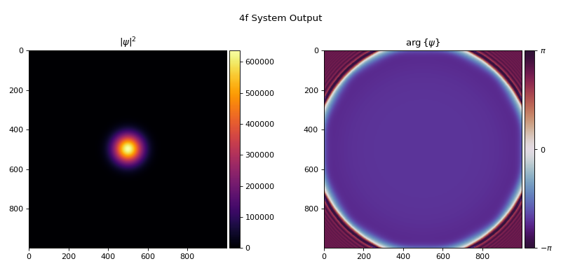
measure_at_z() — measure at a z position with the input grid:

input_field = Field(gaussian(shape, waist_radius=1e-3), z=0)
output = system.measure_at_z(input_field, z=4 * f)
output.visualize(title="4f System Output")

measure() — full control over the output grid:

output = system.measure(
    input_field, shape=(512, 512), z=4 * f, spacing=5e-6, offset=(0, 0),
)

measure_at_plane() — target a PlanarGrid:

from torchoptics import PlanarGrid

output_plane = PlanarGrid(shape=400, z=4 * f, spacing=8e-6)
output = system.measure_at_plane(input_field, output_plane)

Indexing

Systems support indexing, slicing, and iteration:

first = system[0]             # Single element
sub = system[0:2]             # New System from slice
n = len(system)               # Element count

for element in system:
    print(element)

Lens(shape=(1000, 1000), z=2.00e-01, spacing=(1.00e-05, 1.00e-05), offset=(0.00e+00, 0.00e+00), focal_length=2.00e-01)
Lens(shape=(1000, 1000), z=6.00e-01, spacing=(1.00e-05, 1.00e-05), offset=(0.00e+00, 0.00e+00), focal_length=2.00e-01)

Trainable Systems

When elements contain Parameter tensors, the entire system is differentiable end-to-end. See Inverse Design for training loops and optimization.