Elements

Optical elements are planar components that transform a Field at a fixed position along the optical axis. Every element inherits from Element and shares the same grid geometry as Field (shape, spacing, offset, z).

All elements are torch.nn.Module subclasses: they can be moved to the GPU with .to(device), serialized with torch.save(), and composed into System objects.

Modulators

Modulators apply a point-wise complex multiplication to the field:

\[\psi'(x, y) = \mathcal{M}(x, y) \cdot \psi(x, y)\]

where \(\mathcal{M}\) is the modulation profile, a complex mask that reshapes the amplitude, phase, or both.

Element	Profile \(\mathcal{M}(x, y)\)
Modulator	Arbitrary complex: \(\mathcal{M} = m(x,y)\).
PhaseModulator	Phase-only: \(\mathcal{M} = e^{i\phi(x,y)}\).
AmplitudeModulator	Amplitude-only: \(\mathcal{M} = a(x,y) \in [0, 1]\).
PolychromaticPhaseModulator	Wavelength-dependent phase: \(\mathcal{M} = e^{i\,2\pi\,(n(\lambda)-1)\,t/\lambda}\), where \(t\) is the physical thickness and \(n(\lambda)\) is the refractive index.
IdentityElement	Pass-through: \(\mathcal{M} = 1\) (useful as a placeholder in systems).

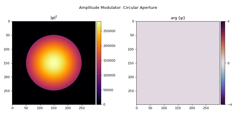
An AmplitudeModulator with a circular mask blocks everything outside the aperture radius:

import math
import torch
import torchoptics
from torchoptics import Field
from torchoptics.elements import AmplitudeModulator, CylindricalLens, Lens, PhaseModulator
from torchoptics.profiles import circle, gaussian

torchoptics.set_default_spacing(10e-6)
torchoptics.set_default_wavelength(700e-9)
shape = 300
beam = Field(gaussian(shape, waist_radius=1.5e-3))

amp_mod = AmplitudeModulator(circle(shape, radius=1e-3), z=0)
amp_mod(beam).visualize(title="Amplitude Modulator: Circular Aperture")

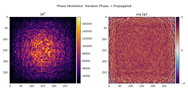
A PhaseModulator leaves the intensity unchanged but alters the phase. After propagation the phase variations produce spatially structured output:

torch.manual_seed(0)
phase_mod = PhaseModulator(torch.randn(shape, shape), z=0)
phase_mod(beam).propagate_to_z(0.2).visualize(title="Phase Modulator: Random Phase → Propagated")

To make a modulator learnable, wrap its profile in torch.nn.Parameter:

from torch.nn import Parameter

trainable_phase = PhaseModulator(Parameter(torch.zeros(300, 300)), z=0)

See Inverse Design for complete optimization workflows.

Polychromatic Modulator

PolychromaticPhaseModulator represents a physical refractive element with a thickness profile \(t(x, y)\) and refractive index \(n(\lambda)\). The same physical element produces different phase shifts at different wavelengths:

\[\phi(x, y, \lambda) = \frac{2\pi}{\lambda}\bigl(n(\lambda) - 1\bigr)\,t(x, y)\]

from torchoptics.elements import PolychromaticPhaseModulator
from torchoptics.profiles import blazed_grating

thickness = blazed_grating(300, period=100e-6, height=700e-9)

# Constant refractive index
grating = PolychromaticPhaseModulator(thickness, n=1.5, z=0)

# Dispersive medium: refractive index as a callable of wavelength
def sellmeier(wl):
    return 1.5 + 0.01e-12 / wl**2  # simplified example

grating_dispersive = PolychromaticPhaseModulator(thickness, n=sellmeier, z=0)

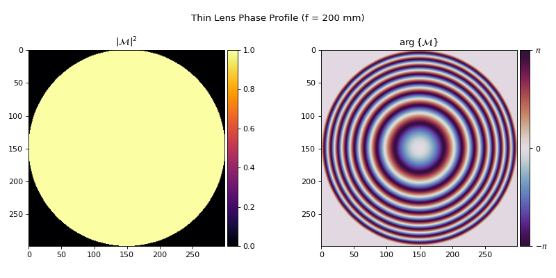
Lenses

Lens models a thin lens with focal length \(f\). It applies a quadratic phase factor within a circular aperture of radius \(R\) (half the lens’s physical extent):

\[\mathcal{M}(x, y) = \operatorname{circ}\!\left(\frac{r}{R}\right) \cdot \exp\!\left(-i \frac{\pi}{\lambda f}(x^2 + y^2)\right)\]

where \(r = \sqrt{x^2 + y^2}\). The phase is wavelength-dependent, matching the behavior of a real refractive lens.

lens = Lens(shape, focal_length=200e-3, z=0)
lens.visualize(title="Thin Lens Phase Profile (f = 200 mm)")

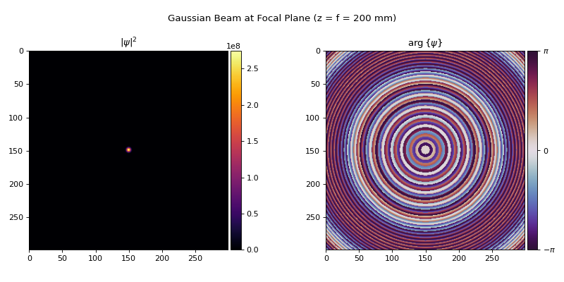
Applying the lens to a Gaussian beam and propagating to the focal plane concentrates the beam into a diffraction-limited spot:

focused = lens(beam).propagate_to_z(200e-3)
focused.visualize(title="Gaussian Beam at Focal Plane (z = f = 200 mm)")

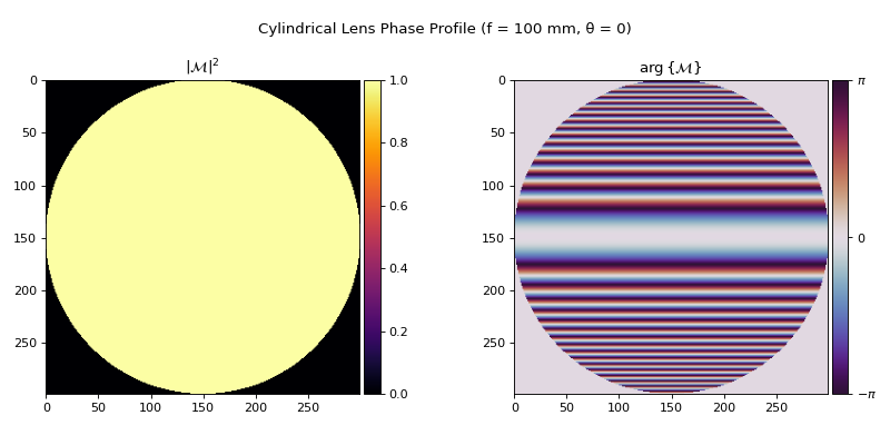
CylindricalLens focuses along a single transverse axis at orientation angle \(\theta\), leaving the perpendicular axis unchanged:

cyl_lens = CylindricalLens(shape, focal_length=100e-3, theta=0, z=0)
cyl_lens.visualize(title="Cylindrical Lens Phase Profile (f = 100 mm, θ = 0)")

Detectors

Detectors convert a field into an intensity measurement, returning a tensor rather than a field. They are natural endpoints for differentiable pipelines: gradients flow back through the detector into upstream elements.

Detector returns the power per grid cell \(P_{i,j} = I_{i,j} \cdot \Delta A\):

from torchoptics.elements import Detector

detector = Detector(shape, z=0.5)
power_map = detector(field)  # Tensor of shape (H, W)

LinearDetector applies a (C, H, W) weight tensor and integrates the field intensity against each weight, producing C scalar output channels, analogous to torch.nn.Linear but operating over 2D spatial intensity maps:

from torchoptics.elements import LinearDetector

weight = torch.randn(10, 300, 300)
lin_detector = LinearDetector(weight, z=0.5)
outputs = lin_detector(field)  # Tensor of shape (10,)

The weight tensor can be made learnable with torch.nn.Parameter, enabling end-to-end optimization of the detector’s spatial selectivity.

Beam Splitters

BeamSplitter models a lossless beam splitter via the transfer matrix:

\[\begin{split}\tau = e^{i\phi_0} \begin{bmatrix} \sin\theta\,e^{i\phi_r} & \cos\theta\,e^{-i\phi_t} \\ \cos\theta\,e^{i\phi_t} & -\sin\theta\,e^{-i\phi_r} \end{bmatrix}\end{split}\]

Setting \(\theta = \pi/4\) gives a 50/50 splitter. The element accepts one or two input fields: a single input acts as a splitter; two inputs recombine them (e.g., at the second beam splitter in a Mach-Zehnder interferometer):

from torchoptics.elements import BeamSplitter

# Dielectric 50:50 beam splitter
bs = BeamSplitter(shape, theta=math.pi/4, phi_0=0, phi_r=0, phi_t=0, z=0)

# Splitting: one input → two output fields
output_1, output_2 = bs(field)

# Recombining: two inputs → two output fields
output_1, output_2 = bs(arm_1, arm_2)

Note

The dielectric 50:50 beam splitter uses \(\phi_t = \phi_r = \phi_0 = 0\). The symmetric (Loudon) beam splitter uses \(\phi_t = 0\), \(\phi_r = -\pi/2\), \(\phi_0 = \pi/2\).

Polarization Elements

The following elements operate on polarized fields: fields whose data tensor has shape (..., 3, H, W), where the size-3 dimension holds the \(x\), \(y\), and \(z\) polarization components. See Polarization for how to construct polarized fields.

Each element applies a 3×3 Jones matrix \(J\) at every grid point:

\[\begin{split}\begin{pmatrix} E_x' \\ E_y' \\ E_z' \end{pmatrix} = J(x, y) \begin{pmatrix} E_x \\ E_y \\ E_z \end{pmatrix}\end{split}\]

Polarizers

LinearPolarizer transmits the field component along angle \(\theta\) and blocks the orthogonal component:

\[\begin{split}J = \begin{bmatrix} \cos^2\theta & \cos\theta\sin\theta & 0 \\ \cos\theta\sin\theta & \sin^2\theta & 0 \\ 0 & 0 & 1 \end{bmatrix}\end{split}\]

from torchoptics.elements import LinearPolarizer

# x-polarized Gaussian beam
polarized_data = torch.zeros(3, shape, shape, dtype=torch.cdouble)
polarized_data[0] = gaussian(shape, waist_radius=1.5e-3)
polarized_field = Field(polarized_data)

lp = LinearPolarizer(shape, theta=0, z=0)           # passes x-component
lp45 = LinearPolarizer(shape, theta=math.pi/4, z=0) # passes diagonal component

LeftCircularPolarizer and RightCircularPolarizer transmit only the left- or right-hand circular polarization component respectively:

from torchoptics.elements import LeftCircularPolarizer, RightCircularPolarizer

lcp = LeftCircularPolarizer(shape, z=0)
rcp = RightCircularPolarizer(shape, z=0)

PolarizingBeamSplitter splits a polarized field into two outputs, each retaining only one transverse polarization component:

from torchoptics.elements import PolarizingBeamSplitter

pbs = PolarizingBeamSplitter(shape, z=0)
field_x, field_y = pbs(polarized_field)

Waveplates

Waveplates introduce a phase delay \(\phi\) between the fast and slow axes, rotating the polarization state without attenuating the field. The general Waveplate Jones matrix is:

\[\begin{split}J = \begin{bmatrix} \cos^2\theta + e^{i\phi}\sin^2\theta & (1 - e^{i\phi})\cos\theta\sin\theta & 0 \\ (1 - e^{i\phi})\cos\theta\sin\theta & \sin^2\theta + e^{i\phi}\cos^2\theta & 0 \\ 0 & 0 & 1 \end{bmatrix}\end{split}\]

where \(\theta\) is the fast-axis angle and \(\phi\) is the phase delay.

Element	Phase delay \(\phi\)
QuarterWaveplate	\(\phi = \pi/2\): converts linear polarization to circular.
HalfWaveplate	\(\phi = \pi\): rotates linear polarization by \(2\theta\).

from torchoptics.elements import HalfWaveplate, QuarterWaveplate, Waveplate

# General waveplate
wp = Waveplate(shape, phi=math.pi/3, theta=math.pi/4, z=0)

# Quarter waveplate at 45°: converts x-linear to circular
qwp = QuarterWaveplate(shape, theta=math.pi/4, z=0)

# Half waveplate at 22.5°: rotates polarization by 45°
hwp = HalfWaveplate(shape, theta=math.pi/8, z=0)

Polarized Modulators

Polarized modulators apply a spatially-varying Jones matrix, enabling position-dependent polarization transformations. Their profile tensor has shape (3, 3, H, W): a full 3×3 Jones matrix at every grid point.

Element	Profile
PolarizedModulator	Arbitrary complex Jones matrix: shape (3, 3, H, W).
PolarizedPhaseModulator	Phase-only Jones matrix: \(e^{i\phi}\), where phase has shape (3, 3, H, W).
PolarizedAmplitudeModulator	Real-valued amplitude Jones matrix: shape (3, 3, H, W).

from torchoptics.elements import PolarizedModulator, PolarizedPhaseModulator

# Spatially uniform identity Jones matrix (pass-through)
jones = torch.eye(3, dtype=torch.cdouble).view(3, 3, 1, 1).expand(3, 3, shape, shape).contiguous()
pol_mod = PolarizedModulator(jones, z=0)

# Spatially-varying phase shift per Jones component
phase = torch.zeros(3, 3, shape, shape)
pol_phase_mod = PolarizedPhaseModulator(phase, z=0)

Visualization

All modulation elements implement visualize(). Polarized elements accept row and column indices to select a specific Jones matrix component:

element.visualize()       # Scalar element: magnitude and phase
polarizer.visualize(0, 0) # Polarized element: Jones matrix component J[0, 0]