
Profiles#
The torchoptics.profiles module provides functions for generating common spatial profiles.
Each function returns a 2D tensor that can be used as the data argument to
Field or as input to elements like
AmplitudeModulator.
All profile functions accept shape, spacing, and offset arguments. When spacing
is omitted, the global default is used.
import torch
import torchoptics
from torchoptics import visualize_tensor
from torchoptics.profiles import (
  airy_pattern, airy_beam, bessel, binary_grating, blazed_grating, checkerboard,
  circle, cylindrical_lens_phase, gaussian, hermite_gaussian, hexagon,
  laguerre_gaussian, lens_phase, plane_wave_phase, rectangle,
  siemens_star, sinc, sinusoidal_grating, spherical_wave_phase,
  square, triangle, zernike,
)

torchoptics.set_default_spacing(10e-6)
Beam Modes#
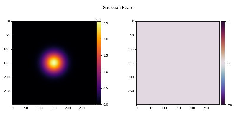
Gaussian#
gaussian() generates the fundamental Gaussian beam:
profile = gaussian(300, waist_radius=500e-6)
visualize_tensor(profile, title="Gaussian Beam")
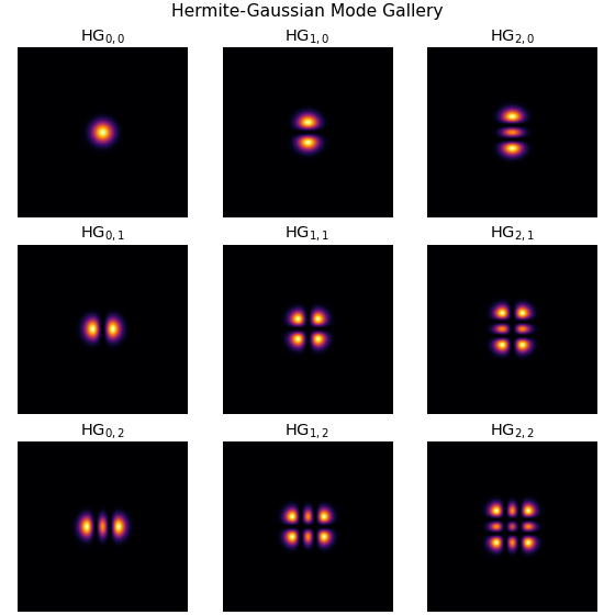
Hermite-Gaussian#
hermite_gaussian() generates higher-order \(\text{HG}_{mn}\)
modes. The indices \(m\) and \(n\) count intensity nodes along the two transverse axes,
producing a rectangular array of \((m+1)(n+1)\) bright lobes:
import matplotlib.pyplot as plt

fig, axes = plt.subplots(3, 3, figsize=(7, 7), constrained_layout=True)
for ax, (m, n) in zip(axes.flat, [(m, n) for n in range(3) for m in range(3)]):
    profile = hermite_gaussian(300, m=m, n=n, waist_radius=250e-6)
    intensity = profile.abs().square()
    ax.imshow(intensity / intensity.max(), cmap="inferno")
    ax.set_title(f"$\\mathrm{{HG}}_{{{m},{n}}}$", fontsize=13)
    ax.axis("off")
plt.suptitle("Hermite-Gaussian Mode Gallery", fontsize=14)
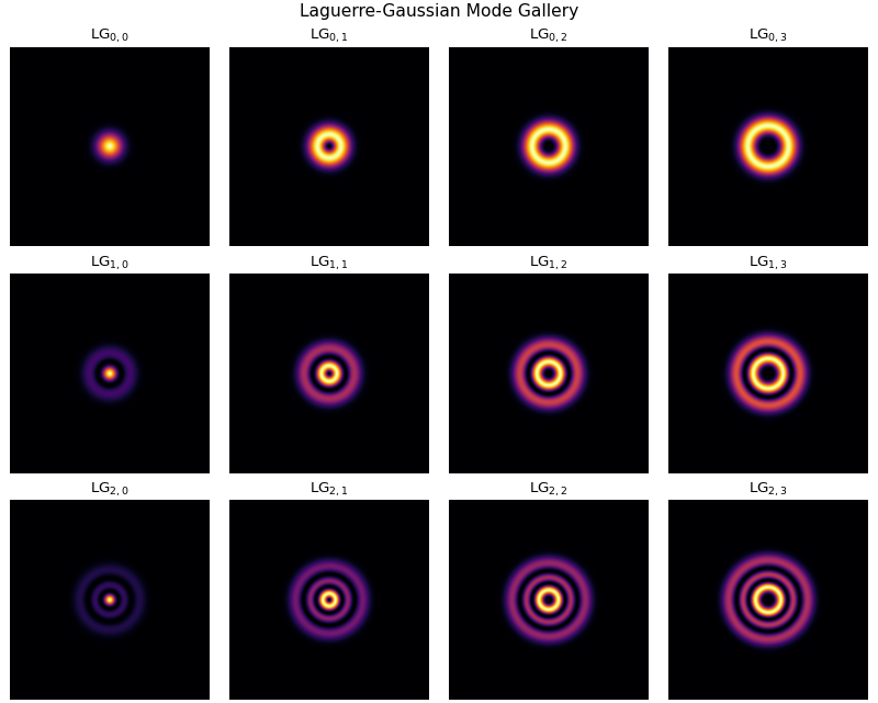
Laguerre-Gaussian#
laguerre_gaussian() generates \(\text{LG}_{p\ell}\) modes.
The radial index \(p\) adds concentric dark rings; the azimuthal index \(\ell\) encodes
the topological charge of the helical phase front \(e^{i\ell\phi}\), which carries orbital
angular momentum of \(\ell\hbar\) per photon:
import matplotlib.pyplot as plt

fig, axes = plt.subplots(3, 4, figsize=(10, 8), constrained_layout=True)
for ax, (p, l) in zip(axes.flat, [(p, l) for p in range(3) for l in range(4)]):
    profile = laguerre_gaussian(300, p=p, l=l, waist_radius=250e-6)
    intensity = profile.abs().square()
    ax.imshow(intensity / intensity.max(), cmap="inferno")
    ax.set_title(f"$\\mathrm{{LG}}_{{{p},{l}}}$", fontsize=12)
    ax.axis("off")
plt.suptitle("Laguerre-Gaussian Mode Gallery", fontsize=14)
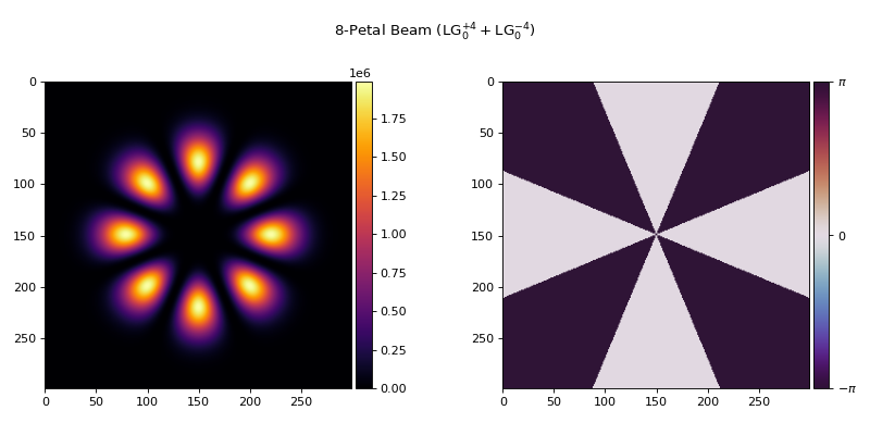
Superpositions of counter-rotating vortices \(\mathrm{LG}_{0}^{+\ell} + \mathrm{LG}_{0}^{-\ell}\) produce \(2|\ell|\) intensity petals through azimuthal interference:
petal = laguerre_gaussian(300, p=0, l=4, waist_radius=500e-6) \
    + laguerre_gaussian(300, p=0, l=-4, waist_radius=500e-6)
visualize_tensor(petal, title="8-Petal Beam ($\\mathrm{LG}_{0}^{+4} + \\mathrm{LG}_{0}^{-4}$)")
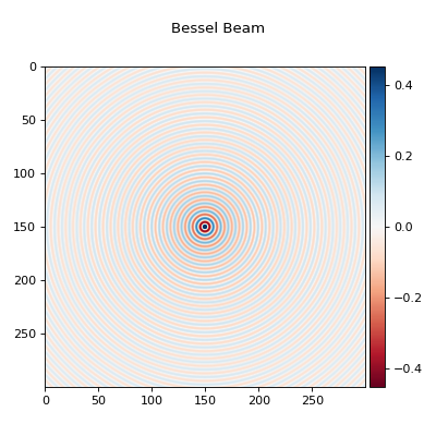
Bessel#
bessel() generates non-diffracting Bessel beams
\(J_0(k r \sin\theta)\):
profile = bessel(300, cone_angle=0.01, wavelength=700e-9)
vmax = profile.abs().max() * 0.5
visualize_tensor(profile, title="Bessel Beam", vmin=-vmax, vmax=vmax, cmap="RdBu")
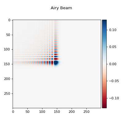
Airy Beam#
airy_beam() generates a truncated 2D Airy beam,
which combines the Airy function with an exponential truncation factor to keep
the energy finite while preserving the characteristic self-accelerating lobe:
profile = airy_beam(300, scale=50e-6, truncation=0.05)
vmax = profile.abs().max().item() * 0.5
visualize_tensor(profile, title="Airy Beam", vmin=-vmax, vmax=vmax, cmap="RdBu")
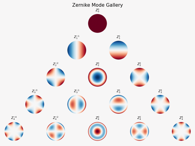
Zernike Modes#
zernike() generates Zernike polynomials
\(Z_n^m(\rho, \theta)\) for wavefront aberrations. The indices \(n\)
and \(m\) determine the radial and angular structure, making these modes a
standard basis for circular pupils and optical aberration analysis:
from matplotlib.gridspec import GridSpec

cmap = plt.get_cmap("RdBu_r")
fig = plt.figure(figsize=(8, 6), facecolor=cmap(0.5))
gs = GridSpec(5, 9, figure=fig, hspace=0.15, wspace=0.05)
fig.subplots_adjust(left=0.02, right=0.98, top=0.92, bottom=0.02)

for n in range(5):
    for i, m in enumerate(range(-n, n + 1, 2)):
        profile = zernike(300, n=n, m=m, radius=1.4e-3)
        ax = fig.add_subplot(gs[n, (4 - n) + 2 * i])
        vmax = profile.abs().max().item()
        ax.imshow(profile, cmap=cmap, vmin=-vmax, vmax=vmax)
        ax.set_title(f"$Z_{{{n}}}^{{{m}}}$", fontsize=9)
        ax.axis("off")
plt.suptitle("Zernike Mode Gallery", fontsize=14)
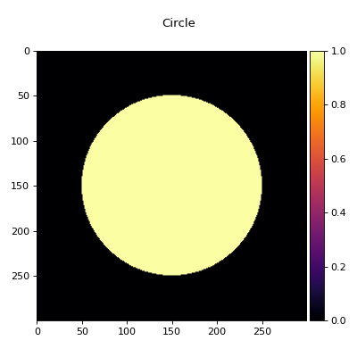
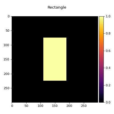
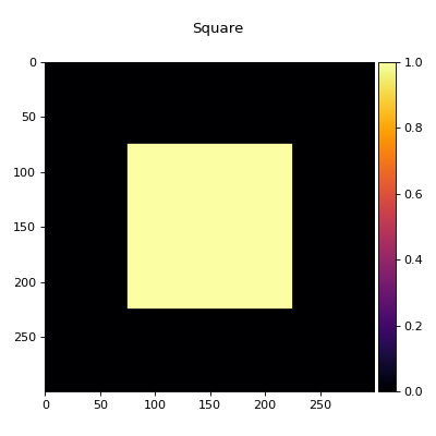
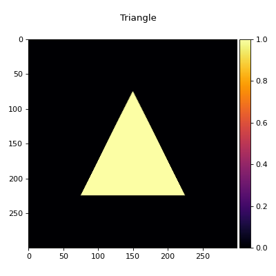
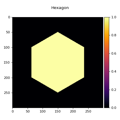
Geometric Apertures#
Binary aperture masks (1 inside, 0 outside):
Function |
Description |
|---|---|
Circular aperture with given |
|
Rectangular aperture with side lengths |
|
Square aperture with side length |
|
Triangular aperture with given |
|
Regular hexagon with circumradius |
|
Regular octagon with circumradius |
|
Regular N-sided polygon with circumradius |
profile = circle(300, radius=1e-3)
visualize_tensor(profile, title="Circle")
profile = rectangle(300, side=(1.5e-3, 0.8e-3))
visualize_tensor(profile, title="Rectangle")
profile = square(300, side=1.5e-3)
visualize_tensor(profile, title="Square")
profile = triangle(300, base=1.5e-3, height=1.5e-3)
visualize_tensor(profile, title="Triangle")
profile = hexagon(300, radius=1e-3)
visualize_tensor(profile, title="Hexagon")
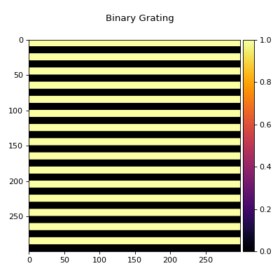
Gratings#
Periodic profiles along a configurable direction:
Function |
Description |
|---|---|
Square-wave grating with configurable duty cycle. |
|
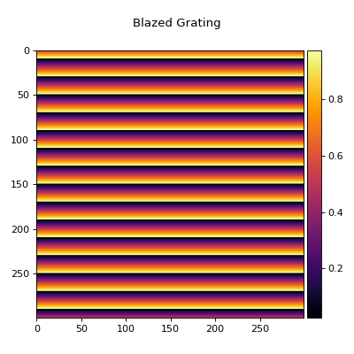
Sawtooth (linearly ramped) grating. |
|
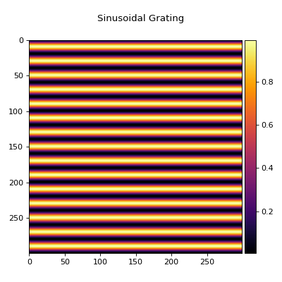
Smooth sinusoidal grating. |
profile = binary_grating(300, period=200e-6)
visualize_tensor(profile, title="Binary Grating")
profile = blazed_grating(300, period=200e-6)
visualize_tensor(profile, title="Blazed Grating")
profile = sinusoidal_grating(300, period=200e-6)
visualize_tensor(profile, title="Sinusoidal Grating")
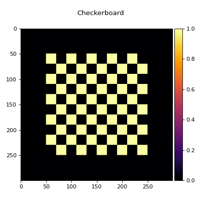
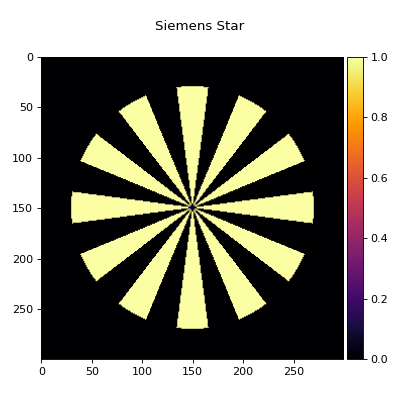
Test Patterns#
Function |
Description |
|---|---|
Tiled checkerboard pattern. |
|
Spoke-based resolution target. |
profile = checkerboard(300, tile_length=200e-6, num_tiles=10)
visualize_tensor(profile, title="Checkerboard")
profile = siemens_star(300, num_spokes=24, radius=1.2e-3)
visualize_tensor(profile, title="Siemens Star")
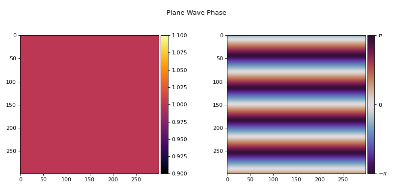
Wave Phases#
Real-valued phase tensors representing the spatial phase of a wavefront in radians. Wrap in
torch.exp(1j * phase) to obtain the complex field amplitude, or pass directly to
PhaseModulator to apply the phase as a modulation element:
Function |
Description |
|---|---|
Tilted plane wave with polar angle \(\theta\) and azimuthal angle \(\phi\). |
|
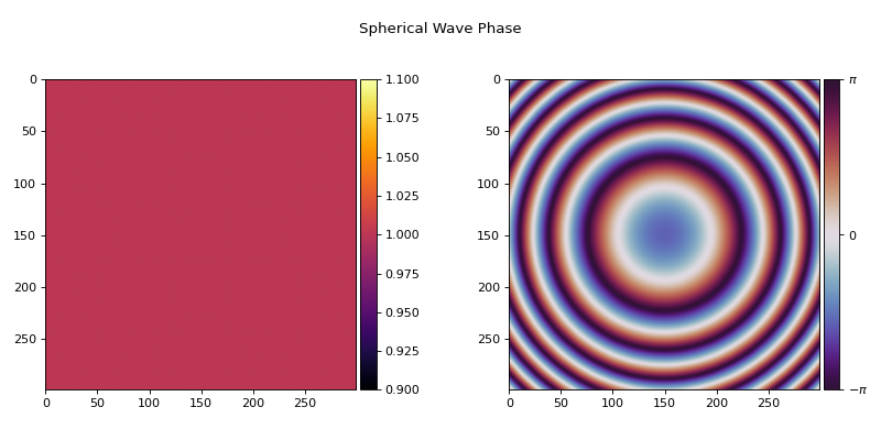
Diverging spherical wave from a point source. |
|
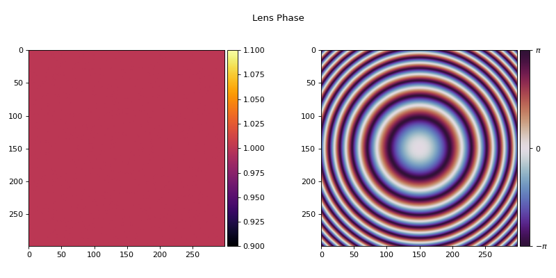
Quadratic thin-lens phase profile. |
|
Quadratic phase in one direction. |
field = torch.exp(1j * plane_wave_phase(300, theta=0.001, wavelength=700e-9))
visualize_tensor(field, title="Plane Wave Phase")
field = torch.exp(1j * spherical_wave_phase(300, z=0.5, wavelength=700e-9))
visualize_tensor(field, title="Spherical Wave Phase")
field = torch.exp(1j * lens_phase(300, focal_length=300e-3, wavelength=700e-9))
visualize_tensor(field, title="Lens Phase")
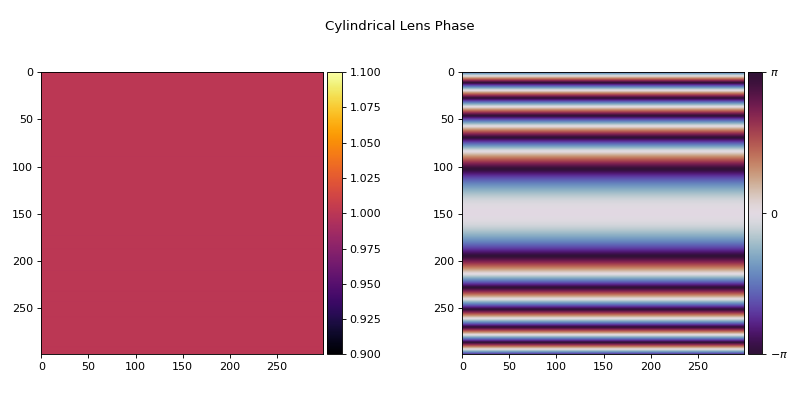
field = torch.exp(1j * cylindrical_lens_phase(300, focal_length=300e-3, wavelength=700e-9))
visualize_tensor(field, title="Cylindrical Lens Phase")
Special Functions#
Function |
Description |
|---|---|
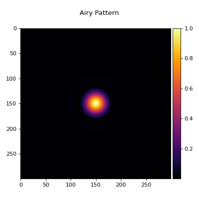
Airy pattern \(\bigl(2J_1(r/a)/(r/a)\bigr)^2\). |
|
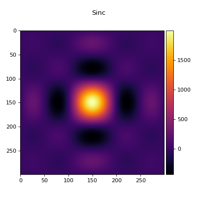
2D sinc function (Fourier transform of a rectangle). |
profile = airy_pattern(300, scale=100e-6)
visualize_tensor(profile, title="Airy Pattern", vmax=1)
profile = sinc(300, scale=(500e-6, 500e-6))
visualize_tensor(profile, title="Sinc")
Coherence Functions#
4D tensors representing the mutual coherence function \(\Gamma(x_1, y_1, x_2, y_2)\) for partially coherent light (see Spatial Coherence):
Function |
Description |
|---|---|
General Schell model with custom intensity and coherence functions. |
|
Gaussian Schell model with Gaussian intensity and coherence. |
Using Profiles with Elements#
Profiles plug directly into elements:
import math
from torchoptics.elements import AmplitudeModulator, PhaseModulator
from torchoptics.profiles import circle, blazed_grating

aperture = AmplitudeModulator(circle(300, radius=1e-3), z=0.1)
grating = PhaseModulator(blazed_grating(300, period=100e-6, height=2 * math.pi), z=0.2)