
Fields#
The Field class is the central object in TorchOptics: a complex-valued
wavefront sampled on a 2D planar grid at a position along the optical axis.
Creating a Field#
Construct a Field from a 2D complex tensor. If spacing or
wavelength are omitted, the global defaults are used (see Configuration).
import torch
import torchoptics
from torchoptics import Field
from torchoptics.profiles import gaussian, circle
torchoptics.set_default_spacing(10e-6)
torchoptics.set_default_wavelength(700e-9)
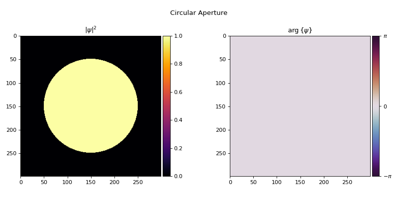
field = Field(circle(300, radius=1e-3))
field.visualize(title="Circular Aperture")
print(field)
Field(shape=(300, 300), z=0.00e+00, spacing=(1.00e-05, 1.00e-05), offset=(0.00e+00, 0.00e+00), wavelength=7.00e-07)
The data tensor must have at least 2 dimensions (H × W). Leading dimensions are treated as
batch dimensions. Fields can be created from profiles functions (see
Profiles) or from arbitrary tensors:
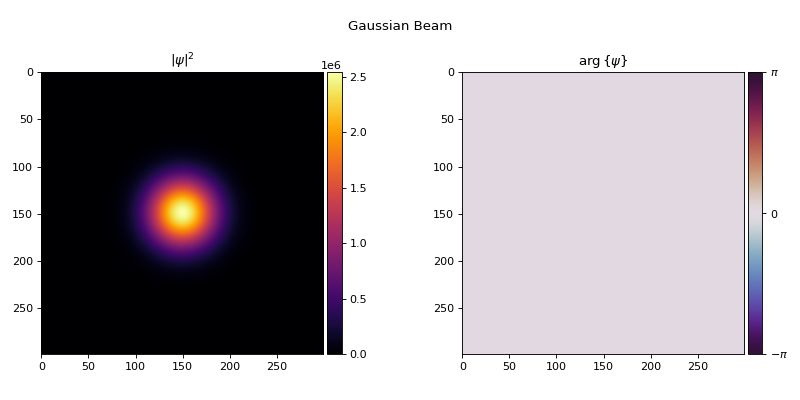
gaussian_field = Field(gaussian(300, waist_radius=500e-6))
gaussian_field.visualize(title="Gaussian Beam")
Grid Geometry#
Every Field inherits from PlanarGrid, which defines
its spatial layout through four properties:
Property |
Type |
Description |
|---|---|---|
|
|
Number of grid points (H, W). |
|
|
Physical distance between adjacent grid points (m). Can differ along the two axes. |
|
|
The (y, x) coordinates of the grid center (m). Default: |
|
|
Position along the optical axis (m). Default: |
Retrieve spatial coordinates and bounds:
x, y = field.meshgrid()     # 2D coordinate arrays
bounds = field.bounds()     # [y_min, y_max, x_min, x_max]
length = field.length()     # Physical extent [Ly, Lx]
Propagation#
Three methods handle free-space propagation (see Propagation for the underlying algorithms):
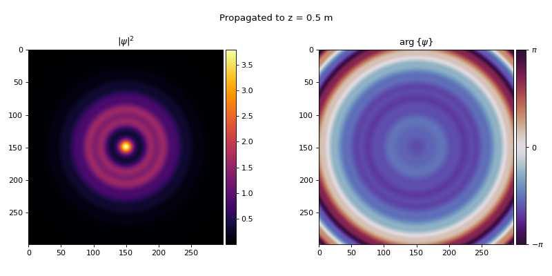
propagate_to_z() — propagate to a new z while preserving grid
geometry:
propagated = field.propagate_to_z(0.5)
propagated.visualize(title="Propagated to z = 0.5 m")
propagate() — full control over the output grid:
output = field.propagate(shape=(512, 512), z=1.0, spacing=5e-6, offset=(100e-6, 0))
propagate_to_plane() — propagate to a
PlanarGrid or element:
from torchoptics import PlanarGrid

target = PlanarGrid(shape=400, z=0.3, spacing=8e-6)
output = field.propagate_to_plane(target)
All three accept optional propagation_method, asm_pad, and interpolation_mode
keyword arguments.
Analysis#
Method |
Description |
|---|---|
Squared magnitude \(|\psi|^2\). |
|
Integrated intensity: \(P = \sum I_{ij}\,\Delta A\). |
|
Intensity-weighted center of mass \((\bar{y}, \bar{x})\). |
|
Intensity-weighted standard deviation along each axis. |
g = Field(gaussian(300, waist_radius=500e-6, offset=(200e-6, 300e-6)))
print(f"Power:    {g.power().item():.4e}")
print(f"Centroid: ({g.centroid()[0].item():.2e}, {g.centroid()[1].item():.2e})")
print(f"Std:      ({g.std()[0].item():.2e}, {g.std()[1].item():.2e})")
Power:    1.0000e+00
Centroid: (2.00e-04, 3.00e-04)
Std:      (2.50e-04, 2.50e-04)
Inner Product#
The overlap integral between two fields is:
inner() returns this as a complex scalar, where \(\psi_1\) is
self and \(\psi_2\) is the argument. Taking the squared magnitude gives the
mode overlap \(|\eta|^2\): a value in \([0, 1]\) when both fields are normalized
to unit power (by Cauchy–Schwarz), and a natural fidelity metric for inverse design
(see Inverse Design):
overlap = field_a.inner(field_b).abs().square()  # |η|² in [0, 1] if both normalized
loss = 1 - overlap
Both fields must share the same geometry (shape, spacing, offset, and z).
Modulation#
Point-wise complex multiplication:
This is the mechanism by which elements transform fields, and can be used to apply arbitrary complex-valued masks directly. The profile may be real (amplitude mask) or complex (phase and amplitude):
# Complex phase mask
profile = torch.exp(1j * torch.randn(300, 300, dtype=torch.double))
modulated = field.modulate(profile)

# Real amplitude mask
from torchoptics.profiles import circle
apertured = field.modulate(circle(300, radius=1e-3))
Normalization and Copying#
normalized = field.normalize()           # Scale to unit power
scaled = field.normalize(2.5)            # Scale to power = 2.5
shifted = field.copy(z=0.5)              # Copy with updated z
rescaled = field.copy(spacing=5e-6)      # Copy with new spacing
Updating Properties#
All registered properties can be updated by direct assignment. Assignments are validated automatically; invalid values raise errors immediately.
field.z = 0.5
field.wavelength = 532e-9
field.spacing = (8e-6, 8e-6)
field.offset = (100e-6, 0)
Element properties work the same way.
Visualization#
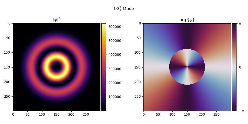
visualize() displays intensity and phase for complex fields:
from torchoptics.profiles import laguerre_gaussian

lg = Field(laguerre_gaussian(300, p=1, l=2, waist_radius=500e-6))
lg.visualize(title="LG$_{1}^{2}$ Mode")
The standalone visualize_tensor() and animate_tensor()
functions work with arbitrary 2D and 3D tensors respectively.
Batched Fields#
The data tensor supports batch dimensions with shape (..., H, W):
batch_data = torch.randn(4, 300, 300, dtype=torch.cdouble)
batch_field = Field(batch_data)

propagated = batch_field.propagate_to_z(0.5)
print(propagated.data.shape)  # torch.Size([4, 300, 300])