Polarization#

Polarized light requires tracking the orientation of the electric field vector, not just its amplitude. TorchOptics extends Field to handle this by representing the field as three complex components along the \(x\), \(y\), and \(z\) directions.

Polarized Fields#

A polarized field has data of shape (3, H, W). In paraxial optics, light travels nearly along the optical axis, so the \(z\) component is typically zero and energy is carried entirely by the transverse components (\(x\) and \(y\)).

Construct a polarized field by placing the desired profile into the appropriate component:

import torch
import torchoptics
from torchoptics import Field
from torchoptics.profiles import gaussian

torchoptics.set_default_spacing(10e-6)
torchoptics.set_default_wavelength(700e-9)
shape = 200

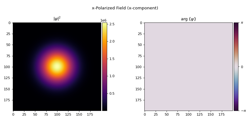
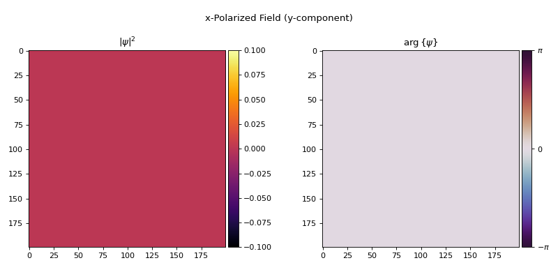
# x-polarized Gaussian beam: only the x-component is non-zero
data = torch.zeros(3, shape, shape, dtype=torch.cdouble)
data[0] = gaussian(shape, waist_radius=500e-6)
x_pol = Field(data)
x_pol.visualize(0, title="x-Polarized Field (x-component)")
x_pol.visualize(1, title="x-Polarized Field (y-component)")
x_pol.visualize(2, title="x-Polarized Field (z-component)")

Jones Calculus#

Polarized elements apply a spatially-varying 3×3 Jones matrix at each grid point:

\[\begin{split}\begin{bmatrix} \psi'_x \\ \psi'_y \\ \psi'_z \end{bmatrix} = \mathbf{J}(x,y) \cdot \begin{bmatrix} \psi_x \\ \psi_y \\ \psi_z \end{bmatrix}\end{split}\]

The full profile has shape (3, 3, H, W), where each \(J_{ij}\) is a 2D tensor over the grid.

Propagation#

Each polarization component propagates independently through free space. All propagation methods work seamlessly with polarized fields; the leading dimension is simply carried through:

propagated = x_pol.propagate_to_z(0.5)
# propagated.data.shape == (3, 200, 200)