Spatial Coherence

Coherent light (e.g. a laser) is described by a single complex field \(\psi(x,y)\). Partially coherent light (LEDs, thermal sources, or spatially filtered broadband sources) requires a statistical description: the mutual coherence function. SpatialCoherence provides this, enabling physically accurate simulation of sources that cannot be modeled by a single wavefront.

Mutual Coherence Function

The mutual coherence function encodes the statistical correlation between two spatial points:

\[\Gamma(x_1, y_1, x_2, y_2) = \langle \psi^*(x_1, y_1) \, \psi(x_2, y_2) \rangle\]

The diagonal \(\Gamma(x, y, x, y) = I(x, y)\) gives the time-averaged intensity. Fully coherent light has \(\Gamma = \psi^* \psi^\top\); incoherent light has \(\Gamma(x_1,y_1,x_2,y_2) = 0\) whenever \((x_1,y_1) \neq (x_2,y_2)\).

SpatialCoherence stores \(\Gamma\) as a 4D complex tensor of shape (H, W, H, W). Calling visualize() displays the time-averaged intensity \(I(x,y) = \Gamma(x,y,x,y)\).

Note

The (H, W, H, W) coherence matrix scales as \(O(N^4)\) in memory. Keep grid sizes small (typically 20–50 points per dimension) or use GPU acceleration for larger problems.

Creating a SpatialCoherence Object

The torchoptics.profiles module provides two functions for constructing common coherence models.

gaussian_schell_model() produces a source with Gaussian intensity and Gaussian coherence:

\[\Gamma(x_1, y_1, x_2, y_2) = \sqrt{I(x_1,y_1)\,I(x_2,y_2)} \cdot \exp\!\left(-\frac{|\mathbf{r}_1-\mathbf{r}_2|^2}{2\sigma_c^2}\right)\]

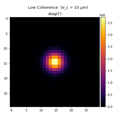
where \(I(x,y) = \frac{2}{\pi w^2}\exp(-2r^2/w^2)\) is the Gaussian intensity with waist \(w\) (normalized to unit power), and \(\sigma_c\) is the coherence width: the length scale over which the field remains correlated. A small \(\sigma_c\) (much less than \(w\)) gives a low-coherence source like an LED; a large \(\sigma_c\) approaches a coherent Gaussian beam:

import torchoptics
from torchoptics import SpatialCoherence, visualize_tensor
from torchoptics.profiles import gaussian_schell_model

torchoptics.set_default_spacing(10e-6)
torchoptics.set_default_wavelength(700e-9)

low_coh = SpatialCoherence(
    gaussian_schell_model(30, waist_radius=40e-6, coherence_width=10e-6)
)
high_coh = SpatialCoherence(
    gaussian_schell_model(30, waist_radius=40e-6, coherence_width=1e-3)
)

low_coh.visualize(title="Low Coherence  (σ_c = 10 µm)")

high_coh.visualize(title="High Coherence  (σ_c = 1 mm)")

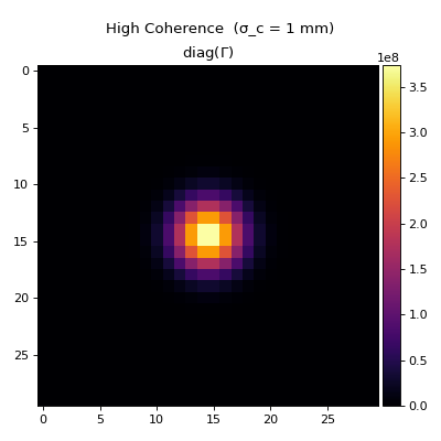
Both sources have the same Gaussian intensity profile; coherence width does not affect the initial intensity distribution, only how the field evolves on propagation.

For custom intensity and coherence shapes, use schell_model() with callable profiles:

import torch
from torchoptics.profiles import schell_model

data = schell_model(
    shape=30,
    intensity_func=lambda x, y: torch.exp(-2 * (x**2 + y**2) / (40e-6)**2),
    coherence_func=lambda dx, dy: torch.exp(-(dx**2 + dy**2) / (2 * (20e-6)**2)),
)
custom_coh = SpatialCoherence(data)

Propagation

Propagation of the coherence function follows \(\Gamma' = U\,\Gamma\,U^\dagger\), where \(U\) is the free-space propagation operator. The same API as coherent fields is used:

propagated = low_coh.propagate_to_z(0.01)

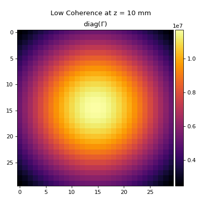
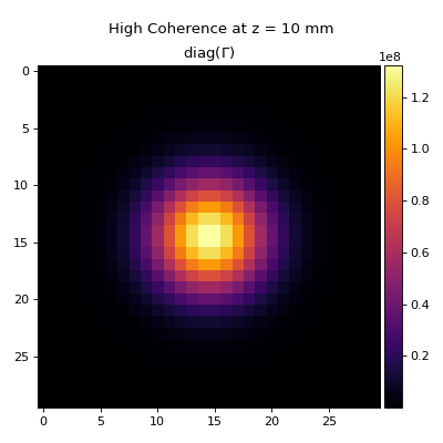
A low-coherence source spreads and loses spatial structure rapidly, while a high-coherence source maintains its beam profile:

low_coh.propagate_to_z(0.01).visualize(title="Low Coherence at z = 10 mm")

high_coh.propagate_to_z(0.01).visualize(title="High Coherence at z = 10 mm")

Intensity, Power, and Modulation

intensity() returns the diagonal of \(\Gamma\) as a (H, W) tensor; power() integrates it:

I = low_coh.intensity()  # shape (H, W)
P = low_coh.power()      # scalar

Scalar modulation applies a complex mask \(\mathcal{M}(x,y)\) to the coherence function:

\[\Gamma'(x_1, y_1, x_2, y_2) = \mathcal{M}^*(x_1, y_1) \cdot \Gamma \cdot \mathcal{M}(x_2, y_2)\]

from torchoptics.profiles import circle

apertured = low_coh.modulate(circle(30, radius=100e-6))